Magnelio

Magnelio is a Python library for full-wave 3D electromagnetic field simulation. Its standard workflow is broadband S-parameter extraction over waveguide ports on arbitrary 3D geometry; the workhorse solver is a time-domain Finite Integration Technique (FIT-TD) engine.

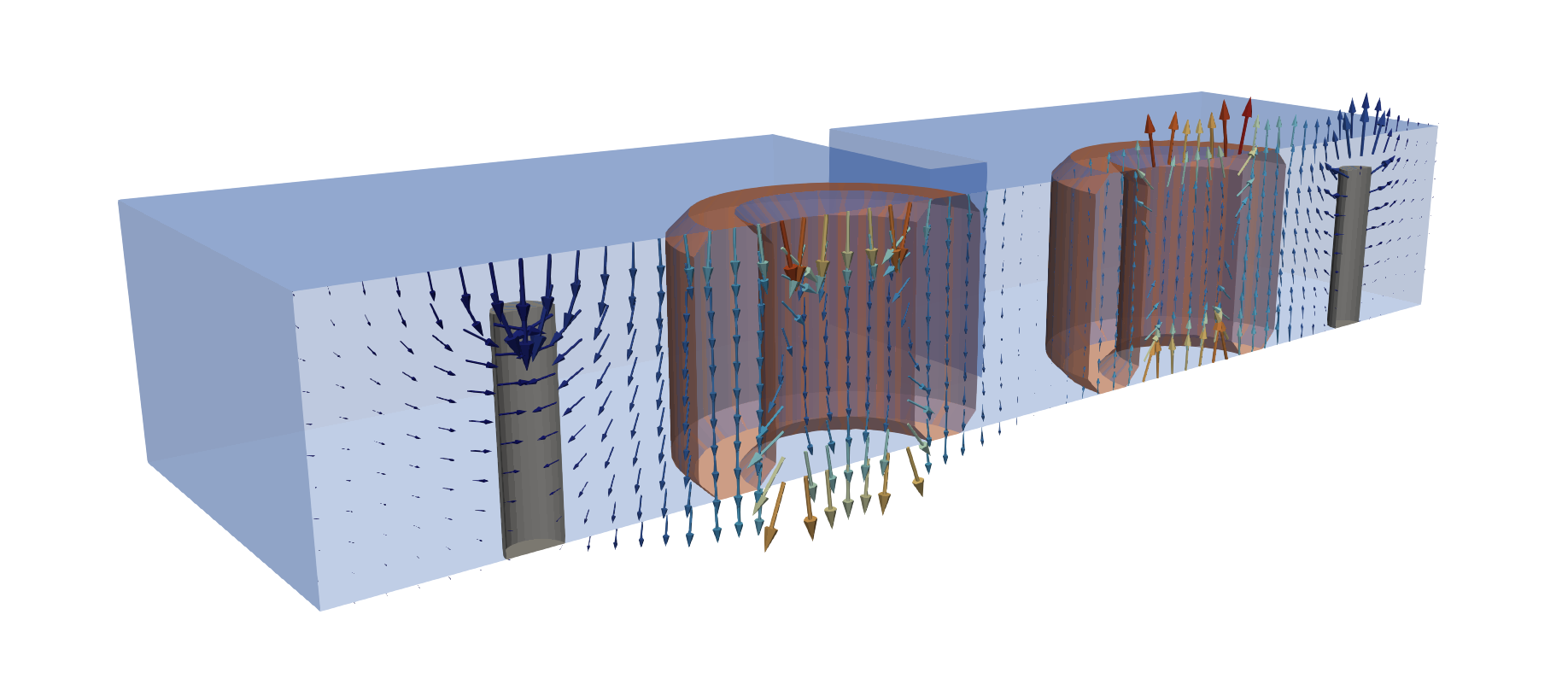
Performance is a design goal, not an afterthought: no field update ever loops over cells in Python. The time-stepping kernels are fused and fully vectorised on three tiers — custom CUDA kernels on the GPU, Numba-compiled multi-threaded kernels on the CPU, and pure array stencils as the portable fallback — so a step runs at compiled-C speed, and models with hundreds of geometric primitives and correspondingly large grids stay tractable.

Features

• FIT time-domain leapfrog solver on a structured non-uniform hexahedral grid, with conformal (sub-cell) material matrices
• NumPy (CPU) and CuPy (CUDA GPU) backends — backend="auto" uses the GPU when available, with CUDA-graph stepping
• Waveguide ports with exact discrete transparent boundaries (DTBC): TEM / QTEM / TE / TM / hybrid modes, multi-mode, declared on the model before meshing; lumped (RLC-backed) ports
• Boundary conditions: PEC, PMC, CPML, periodic, and symmetry planes — declared once on the model, carried by the mesh
• Materials: isotropic and diagonal-anisotropic, pole-residue dispersion for ε(ω)/μ(ω) with built-in vector fitting, conductor losses (perturbative or SIBC wall model), surface roughness (Hammerstad, Huray)
• Geometry: CSG primitives + Boolean operators (a - b, a + b, a & b), chainable transforms, and profile-based construction (loft, sweep, revolve, shell) via pythonocc-core
• Circuit elements embedded in the field solution: thin wires and lumped RLC networks
• Field monitors (time/frequency domain, flux, wall loss), plane-wave source (TF/SF), 3D eigenmode solver
• Antennas: near-to-far-field transform recorded on a Huygens box the monitor places by itself, with image theory for ground planes and symmetry planes — directivity, gain, realized gain, radiated power and efficiency, drawn as polar cuts or a 3D pattern surface
• Project store on disk: streamed results, bit-exact resume, post-processing on the stored data (HDF5 + ParaView/XDMF); every run generates a ready-to-open ParaView session (coloured per-solid geometry, slice planes, normalised field glyphs)
• Interop: Touchstone (.sNp) export and scikit-rf adapter

Installation

From conda-forge, which is the route to take:

conda install -c conda-forge magnelio

New to conda-forge? miniforge3 is the smallest way in; the Anaconda distribution works too.

There is a PyPI package as well:

pip install magnelio

It installs and imports, but it cannot build a mesh from geometry: that needs pythonocc-core (the Python bindings to Open CASCADE Technology), which is published on conda-forge only. Since a model normally starts with geometry, pip is the fallback for environments where conda is not an option, not the way to run simulations.

The CUDA backend is optional on either route: install a cupy matching your CUDA version and backend="auto" picks the GPU up. Without it the solver runs on the CPU.

Working from a source checkout is described in CONTRIBUTING.md.

Quick Start

S-parameters of a WR-90 rectangular waveguide section:

import magnelio as mio
from magnelio import geo, ports

a, b, L = 22.86e-3, 10.16e-3, 40.0e-3   # WR-90 cross-section, length
f_max = 25.0e9

air = mio.Material.air()
model = mio.GeometryModel(background=air)   # walls: PEC by default
model.add(geo.Brick(origin=(0, 0, 0), size=(a, b, L), material=air))
model.add_port(ports.PortWaveguide(name="port1", plane="zmin", n_modes=3))
model.add_port(ports.PortWaveguide(name="port2", plane="zmax", n_modes=3))

mesh = mio.Mesh.from_geometry(
    model, mio.MeshControl(min_nodes_per_wavelength=15), f_max=f_max,
)

analysis = mio.AnalysisScatteringTD(mesh=mesh, f_max=f_max)
print(analysis.solve_ports()["port1"])   # mode table before the run

result = analysis.run(
    excited=[(p, m) for p in ("port1", "port2") for m in range(3)],
)
result.plot_s(("port2", "port1"), ("port1", "port1"))   # |S| over frequency
s21 = result.S("port2", "port1")         # complex S21 on result.f_axis
result.to_touchstone("wr90.s6p")         # 6 channels = 2 ports × 3 modes

Fourteen executable tutorials — from a first parallel-plate line to a dielectric-resonator filter — live in examples/tutorials/; they are the source of the documentation's tutorial series.

Documentation

docs/ holds the Sphinx documentation: the tutorial series, an API reference for the public surface (the core namespace and the domain namespaces, generated from the docstrings) and the technical method chapters — every numerical method with its literature source. Build it locally with:

pip install -e .[docs]
sphinx-build -b html docs docs/_build/html

Reporting bugs

Wrong results, crashes and refused valid input belong in the issue tracker. The bug form asks for the version, the backend and a short script — a script that reproduces the behaviour is what turns a report into a test case.

known-bugs.md is a different thing and not the place to file: it is the developer's record of investigated defects, with the measurements that pin them down, kept in the repository so a code comment can point at an entry.

Development

Magnelio is being built in an AI-assisted workflow ("vibe coding"): the code is written in collaboration with LLM coding agents, with method selection, validation targets and reviews set by the author. Every numerical method is anchored to published literature in the documentation's method chapters, and the test and validation suite — not the authoring process — is the arbiter of correctness.

License

Magnelio is free software, released under the GNU Lesser General Public License v3.0 or later (LGPL-3.0-or-later) — see COPYING and COPYING.LESSER. You may use it from proprietary code; changes to magnelio itself must be published under the same license when distributed.