| 👤 Author | Muhammad Idrees |
|---|---|
| 🎓 Roll No | 23I-0582 |
| 🏛️ Department | Computer Science |
| 🏫 University | FAST-NUCES, Islamabad |
| 📧 Contact | i230582@isb.nu.edu.pk |
| 📄 Report | Technical Report (PDF) |
- Project Overview
- Repository Structure
- Dataset Overview
- Statistical EDA
- Noise Injection
- Model Architecture
- Training
- Evaluation & Results
- Experimental Study
- Discussion
- Setup & Usage
- Academic Report
- References
- License
This repository implements a fully convolutional Denoising Autoencoder (DAE) trained on the CIFAR-10 dataset. The model learns to reconstruct clean 32×32 RGB images from inputs corrupted by Gaussian and Salt-and-Pepper noise, achieving up to 28 dB PSNR on moderate noise levels with only ~182K parameters.
The project includes:
- A deep convolutional encoder-decoder architecture with configurable bottleneck
- Comprehensive statistical EDA of the CIFAR-10 dataset (45+ publication-quality figures)
- Ablation study over noise levels and bottleneck sizes
- A full 10-page LNCS-format academic report
| Noise Configuration | Input PSNR | Output PSNR | SSIM | Quality Gain |
|---|---|---|---|---|
| Gaussian (σ=0.1) | 20.00 dB | 24.62 dB | 0.8225 | +4.62 dB |
| Salt-and-Pepper (p=0.05) | 21.05 dB | 25.84 dB | 0.8013 | +4.79 dB |
All metrics evaluated on 10,000 held-out CIFAR-10 test images.
denoising-autoencoder-cifar10/
│
├── 📁 src/
│   ├── denoising_autoencoder_cifar10.py    # Full DAE training & evaluation pipeline
│   └── cifar_statistics.py                 # Statistical analysis engine (EDA)
│
├── 📁 notebooks/
│   ├── Denoising_Autoencoder_CIFAR_10.ipynb
│   └── Cifar_Statistics.ipynb
│
├── 📁 report/
│   ├── lncs_report.pdf                     # Compiled LNCS-format technical report
│   ├── lncs_report.tex                     # LaTeX source
│   └── 📁 figures/                         # 45+ publication-quality plots
│       ├── fig01_cifar10_samples.png
│       ├── fig02_class_distribution.png
│       ├── fig03_pixel_histograms.png
│       ├── fig04_class_prototypes.png
│       ├── fig05_noise_types_comparison.png
│       ├── fig06_noise_level_progression.png
│       ├── fig07_input_psnr_bars.png
│       ├── fig08_architecture_diagram.png
│       ├── fig09_parameter_analysis.png
│       ├── fig10_training_dashboard.png
│       ├── fig11_denoising_results_grid.png
│       ├── fig12_error_maps.png
│       ├── fig13_metric_distributions.png
│       ├── fig14_per_class_metrics.png
│       ├── fig15_fft_analysis.png
│       ├── fig17_expA_noise_levels.png
│       ├── fig18_expB_bottleneck.png
│       ├── fig19_heatmaps_psnr_ssim.png
│       ├── fig20_radar_chart.png
│       ├── fig21_failure_analysis.png
│       ├── fig22_final_comparison.png
│       └── fig23_results_dashboard.png
│
├── 📁 architecture/
│   └── diagram.svg                         # High-resolution vector architecture diagram
│
├── .gitignore
├── LICENSE
├── requirements.txt
└── README.mdThe CIFAR-10 dataset contains 60,000 color images of size 32×32×3 across 10 balanced classes: airplane, automobile, bird, cat, deer, dog, frog, horse, ship, and truck.
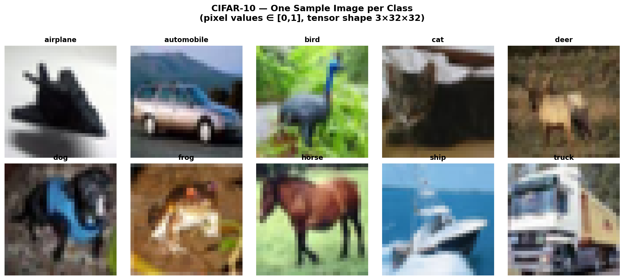
Fig. 1 — One sample image per class from CIFAR-10 (pixel values in [0,1], tensor shape 3×32×32).
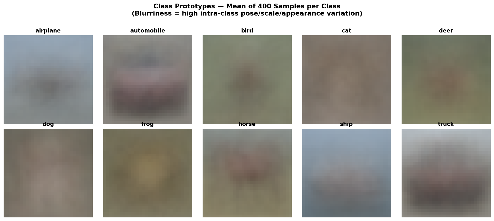
Fig. 2 — Mean (prototype) images per class, computed by averaging 5,000 training images each. Blurriness reflects high intra-class pose/scale/appearance variation.
| Split | Size | Purpose |
|---|---|---|
| Training | 40,000 | Weight updates |
| Validation | 10,000 | Early stopping / best-model selection |
| Test | 10,000 | Final held-out evaluation only |
| Channel | Mean | Std Dev |
|---|---|---|
| Red | 0.4914 | 0.2470 |
| Green | 0.4822 | 0.2435 |
| Blue | 0.4465 | 0.2616 |
| Global | 0.4734 | 0.2516 |
![]()
Fig. 3 — Per-channel pixel value histograms (training set). Red and Green channels are centered near 0.49, while Blue is slightly left-shifted, reflecting the natural color bias of CIFAR-10 scenes.
A comprehensive statistical analysis was performed to characterize the CIFAR-10 dataset before building the denoising model — covering descriptive statistics, distribution testing, correlation analysis, and dimensionality reduction.
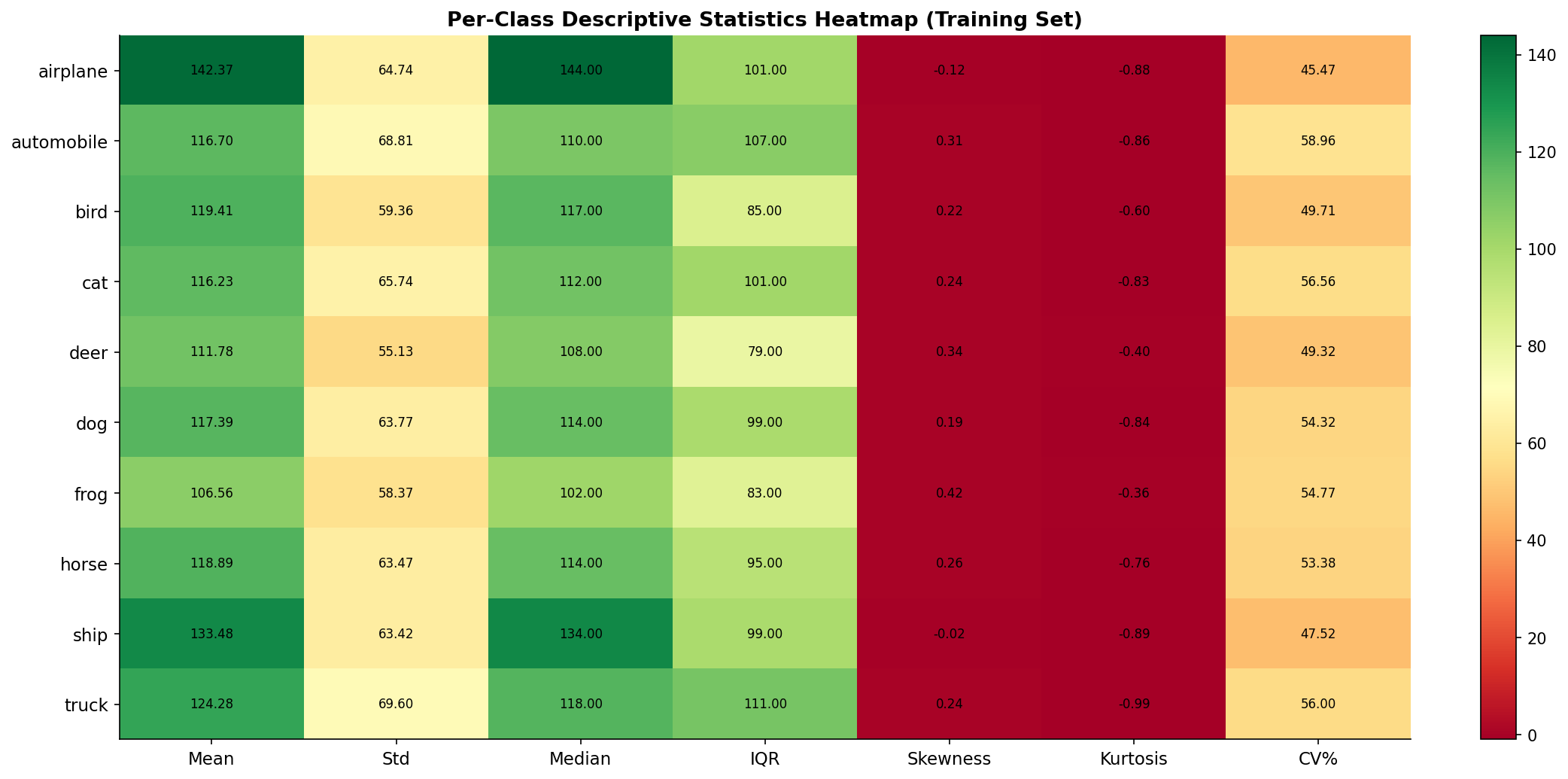
Fig. 4 — Per-class descriptive statistics heatmap (mean, std, median, IQR, skewness, kurtosis, CV%). Color intensity encodes the metric value across all 10 CIFAR-10 classes.
Key Observations:
- Frog has the highest mean pixel value due to dominant green backgrounds
- Cat and Dog exhibit the highest standard deviations, reflecting diverse appearance patterns
- All classes show right-skewed, platykurtic pixel distributions (lighter tails than Gaussian)
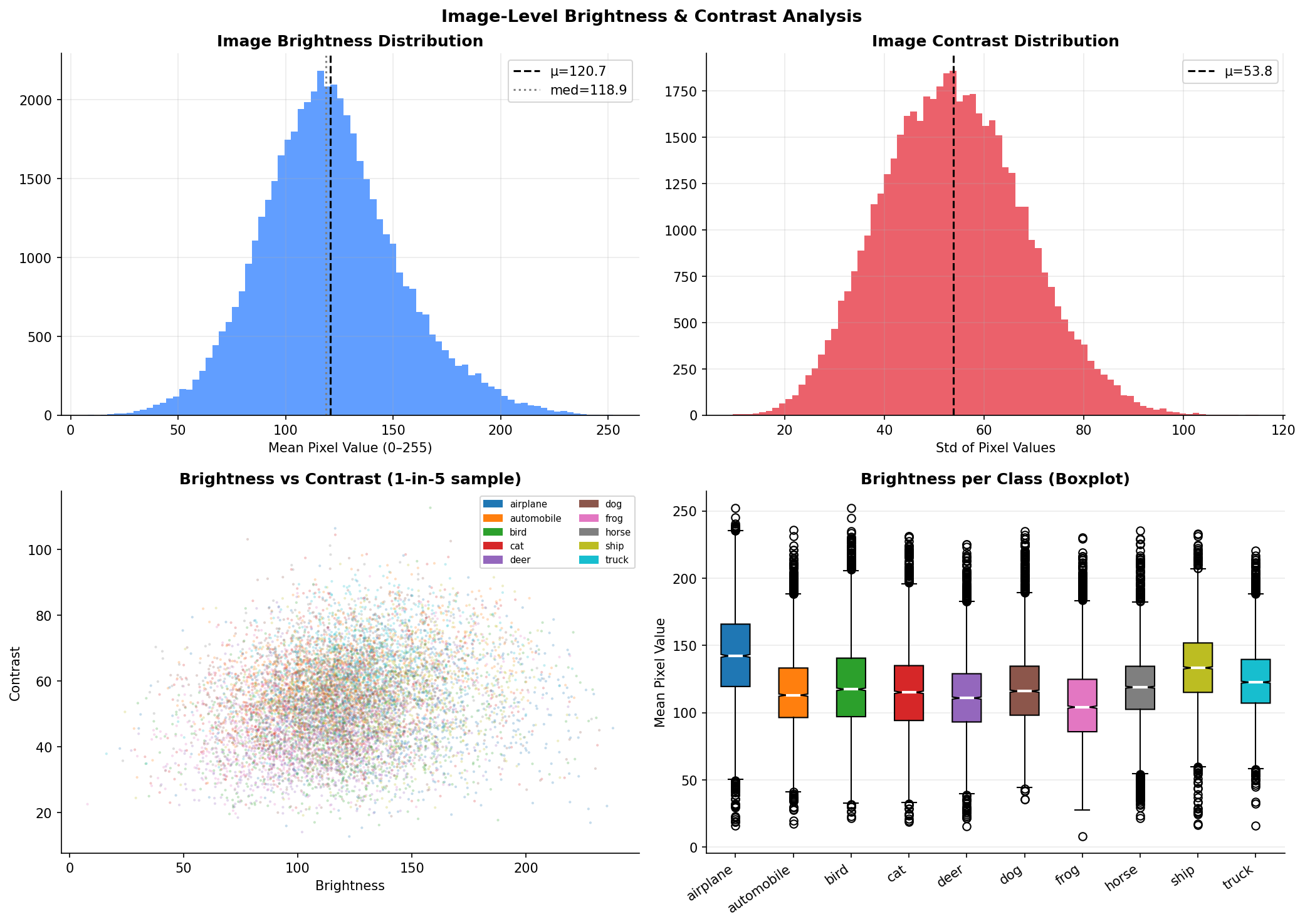
Fig. 5 — Image-level brightness and contrast analysis. Top-left: brightness histogram (μ=120.7, med=118.9). Top-right: contrast histogram (μ=53.8). Bottom-left: brightness vs. contrast scatter by class. Bottom-right: per-class brightness boxplot.
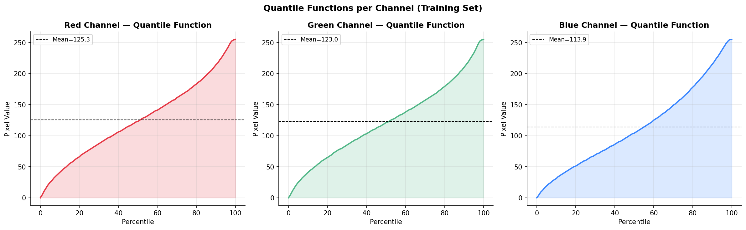
Fig. 6 — Quantile functions per channel (training set). The Red channel has a wider interquartile range than Blue. Extreme pixel values near 0 or 1 are relatively rare across all channels.
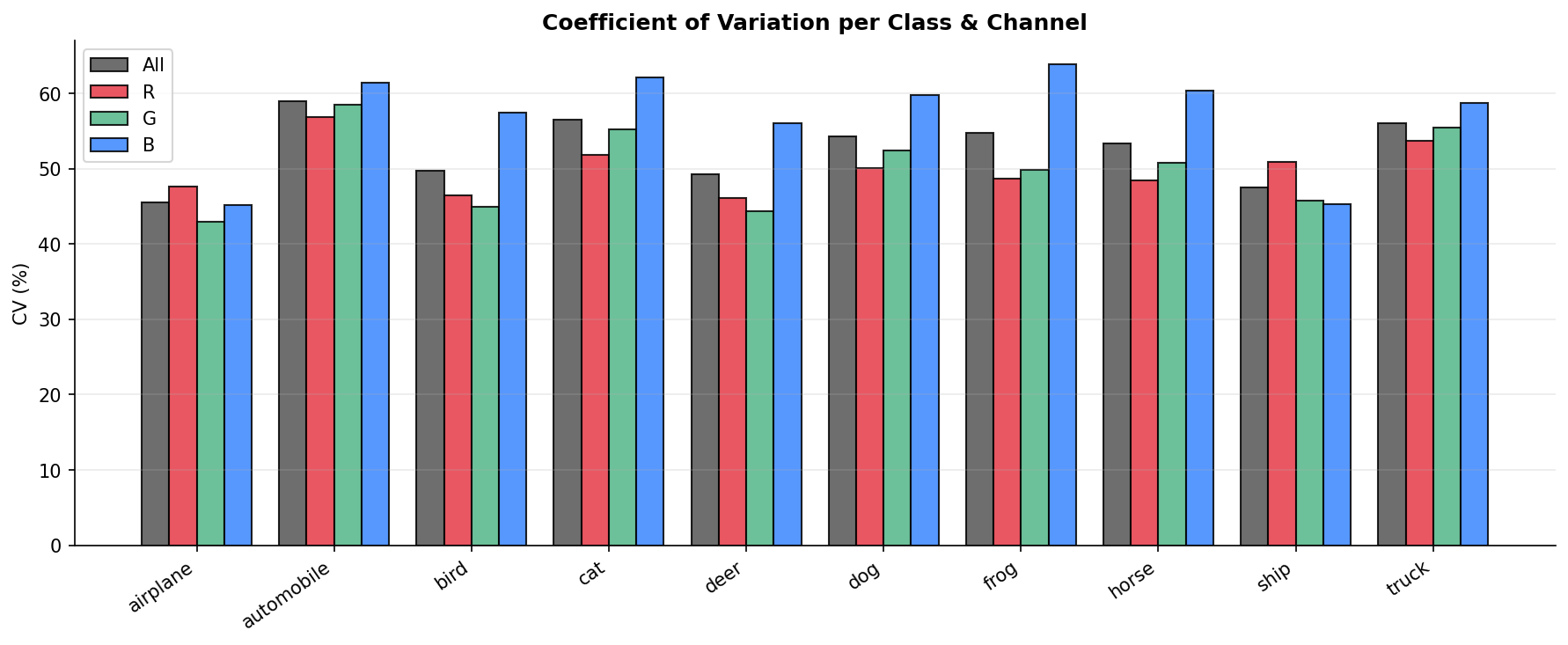
Fig. 7 — Coefficient of Variation (%) per class and color channel. The Blue channel consistently exhibits the highest CV across all classes, indicating it carries the most relative pixel variability.
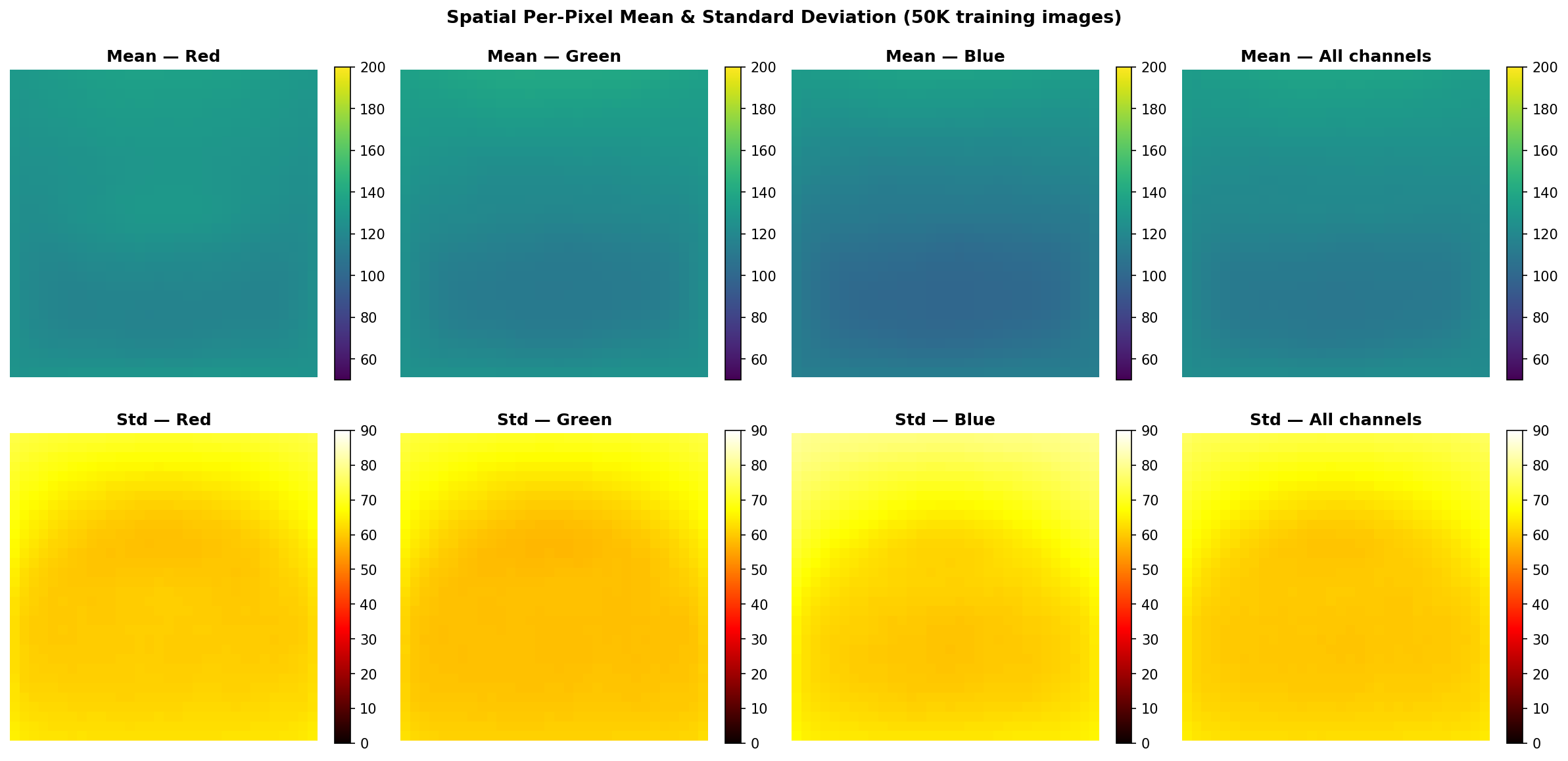
Fig. 8 — Spatial per-pixel mean (top row) and standard deviation (bottom row) maps computed from all 50,000 training images, shown per channel and globally. Center pixels exhibit higher variance — consistent with object-centric image compositions.
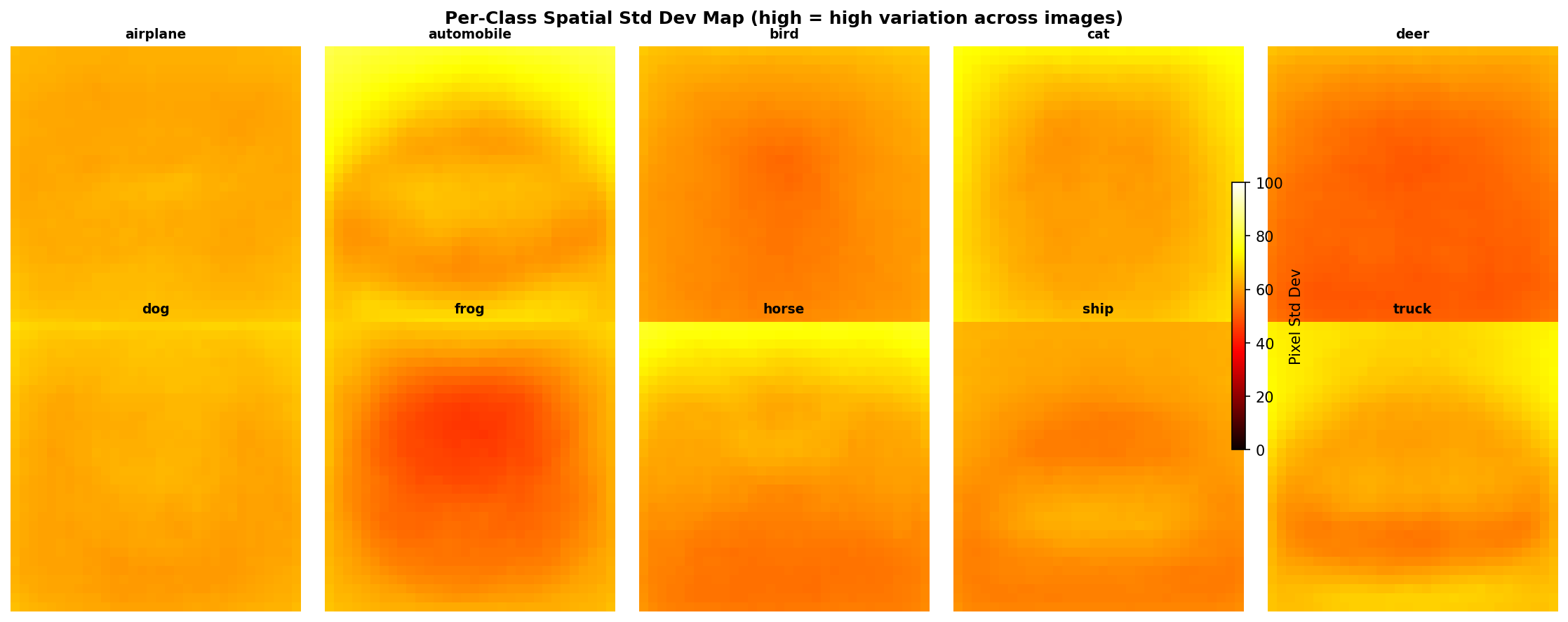
Fig. 9 — Per-class spatial standard deviation maps (high = high variation across images of that class). Vehicle classes (airplane, ship) show concentrated central variance; animal classes exhibit more diffuse spatial patterns.
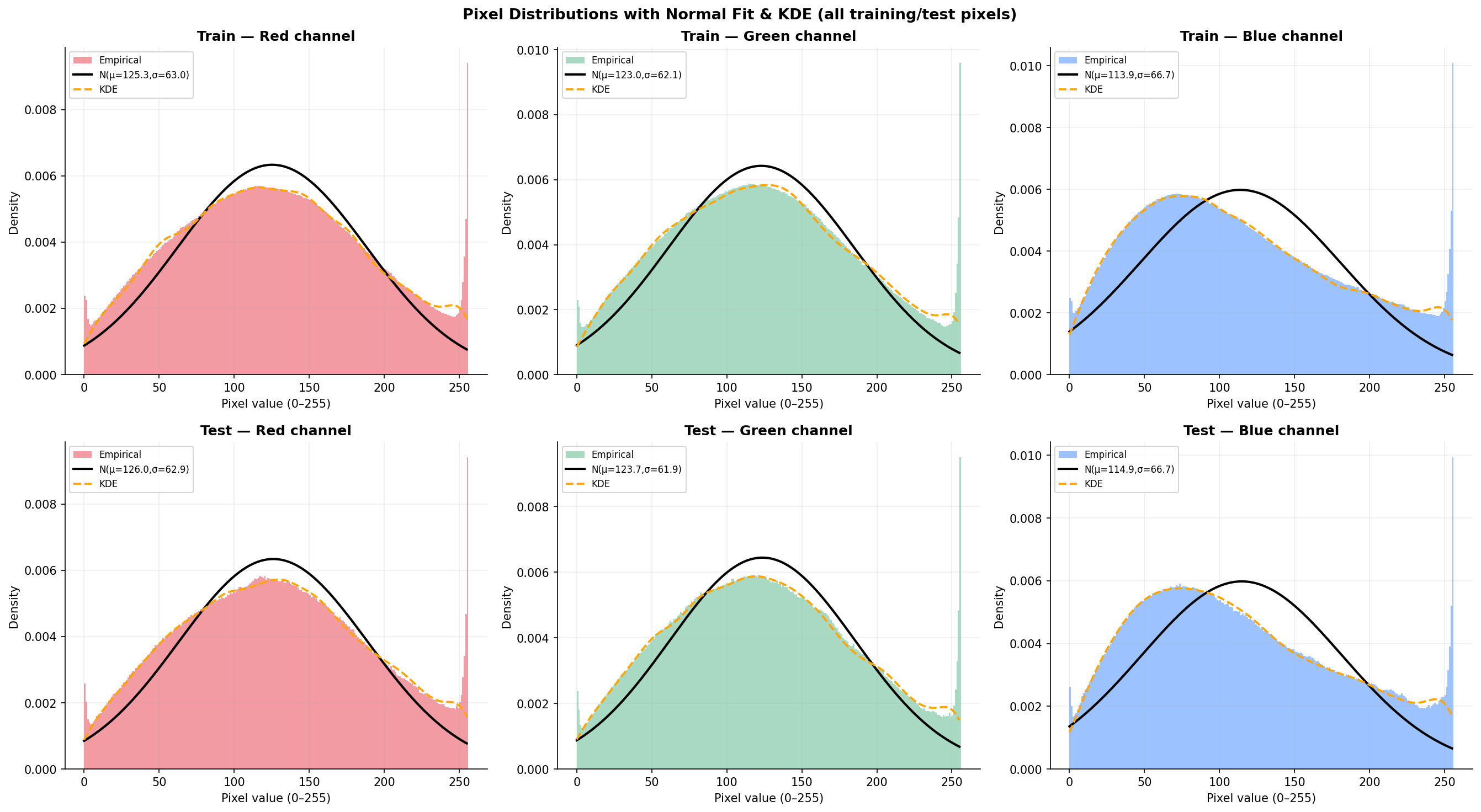
Fig. 10 — Pixel value histograms with fitted Normal distribution and KDE overlays. Top row: training set; Bottom row: test set. The bimodal shape (peaks near 0 and 128) confirms significant deviation from normality across all three channels.
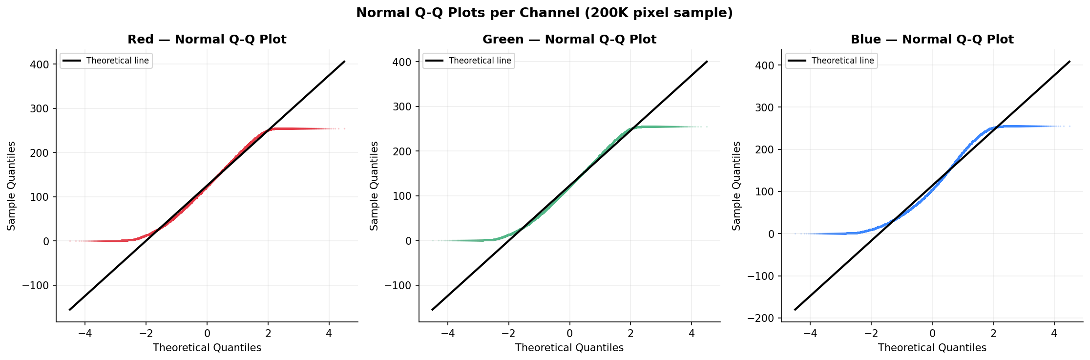
Fig. 11 — Normal Q-Q plots per channel (200K pixel sample). The systematic S-shaped deviation from the diagonal confirms non-normality, with heavy tails evident at both extremes — consistent with the bimodal histogram shapes.
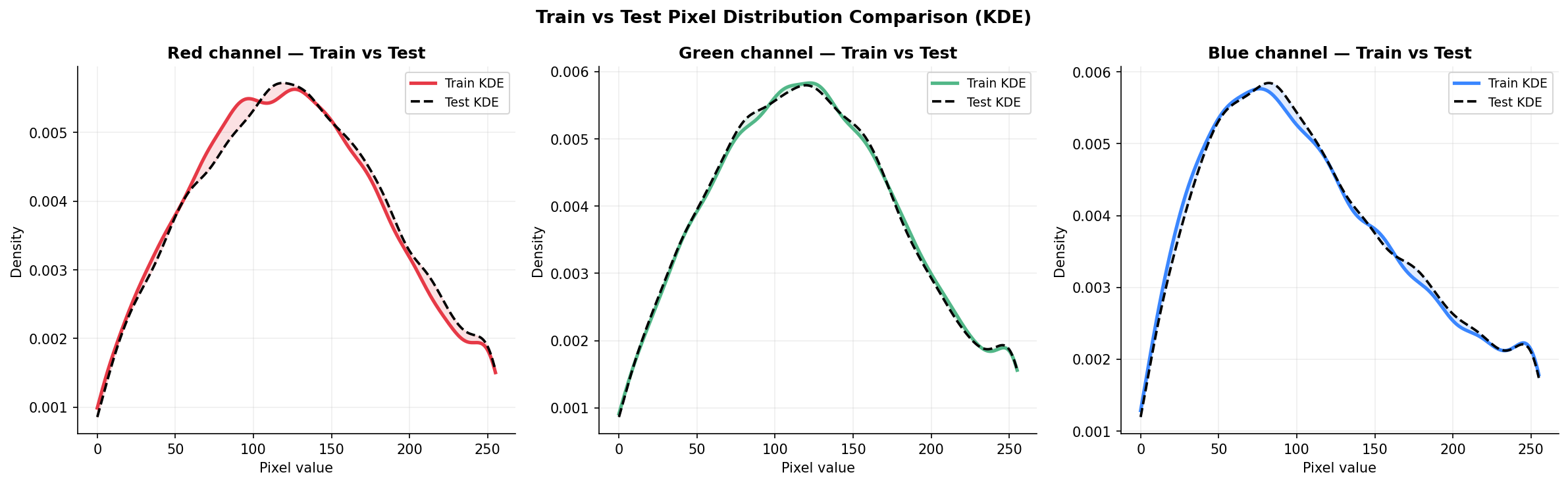
Fig. 12 — Train vs. Test pixel distribution comparison using KDE. Near-perfect overlap between training (solid) and test (dashed) curves validates consistent dataset splitting and confirms the test set is representative.
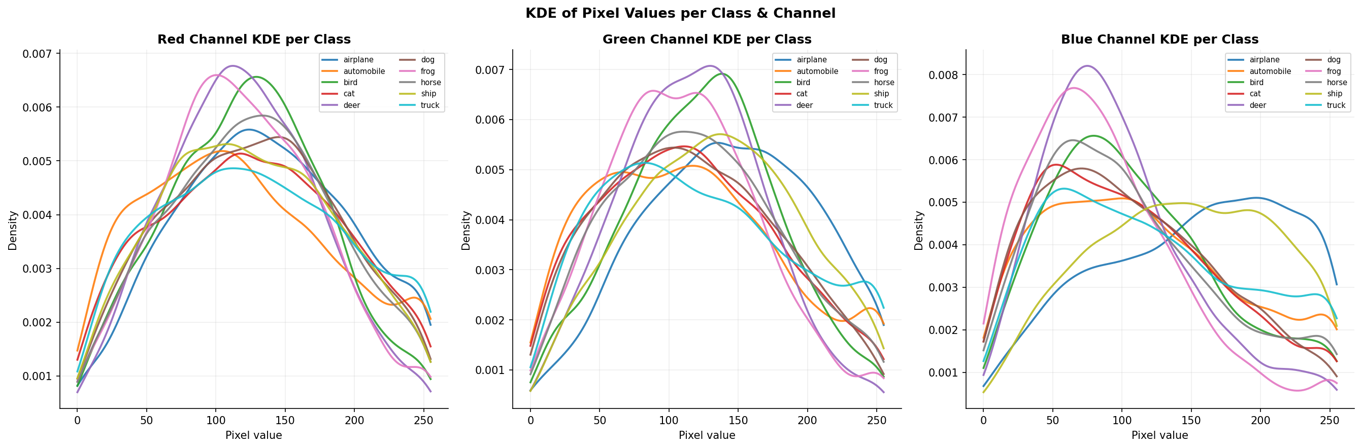
Fig. 13 — KDE of pixel values per class and channel. Classes like "frog" and "deer" dominate higher pixel values (green-shifted); "automobile" and "truck" peak at darker values — capturing class-specific color signatures.
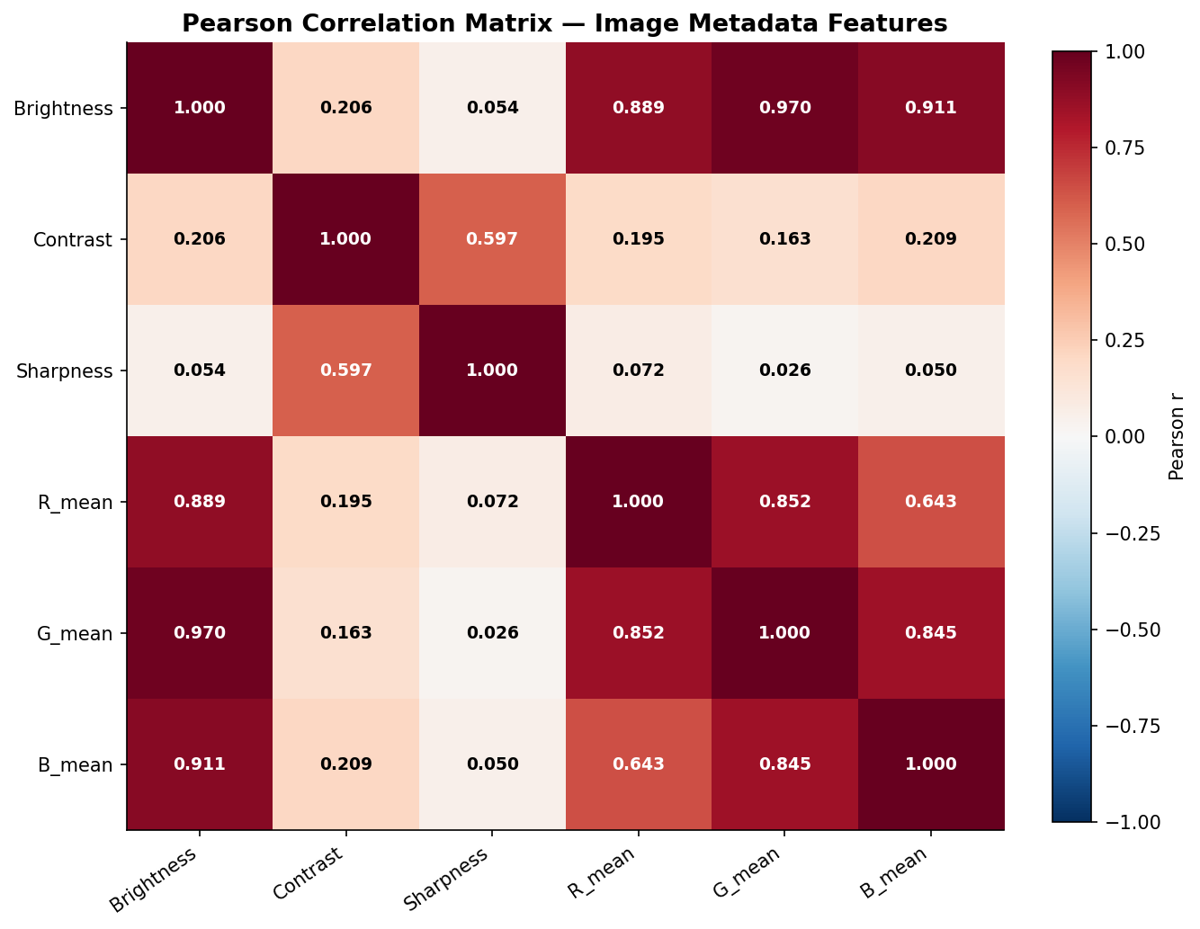
Fig. 14 — Pearson correlation matrix between image metadata features (Brightness, Contrast, Sharpness, R_mean, G_mean, B_mean). Strong R-G-B inter-correlations (r > 0.85) reflect the dominance of luminance variation over chrominance in natural images.

Fig. 15 — Per-class channel correlation analysis (R-G, R-B, G-B). The "frog" class shows weaker R-B correlation due to its distinctive green-dominant colorspace. Vehicle classes show higher, more uniform inter-channel correlations.
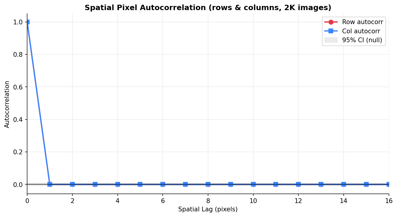
Fig. 16 — Spatial pixel autocorrelation (rows and columns, 2K images). Strong positive correlation between adjacent pixels decays sharply with spatial lag — a key property that convolutional autoencoders exploit during reconstruction.
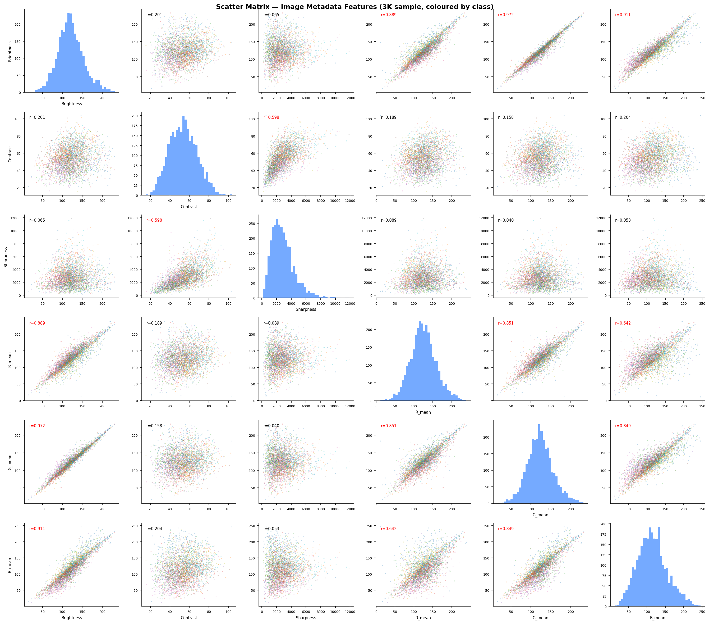
Fig. 17 — R-G-B channel scatter matrix (1K sample, colored by CIFAR-10 class). Ellipsoidal point clouds indicate approximate joint normality at the image level. Class clusters are partially separable in the RGB feature space.
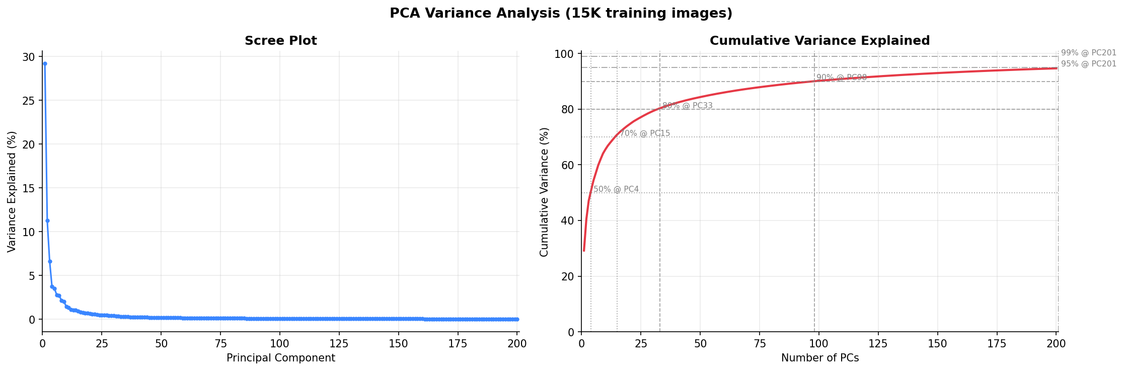
Fig. 18 — PCA scree plot and cumulative explained variance (15K training images). The first 100 components capture ~90% of total variance, demonstrating that CIFAR-10 images reside on a much lower-dimensional manifold than their 3,072-dimensional pixel space suggests.
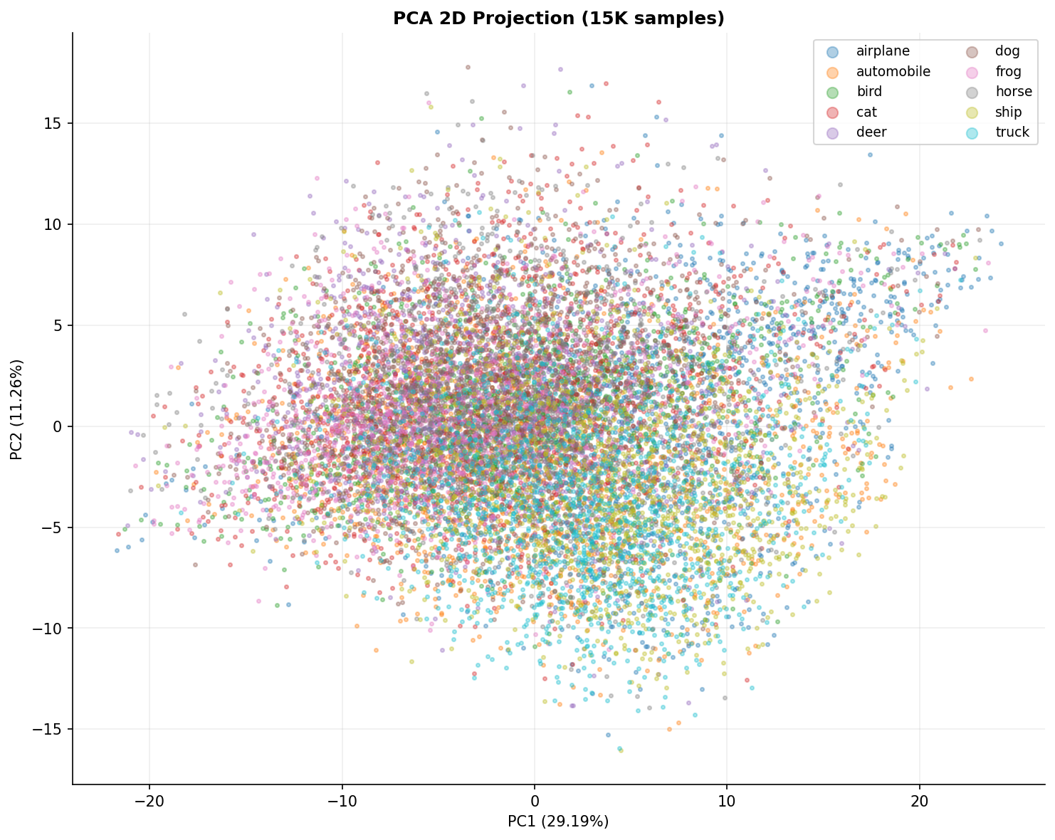
Fig. 19 — 2D PCA projection (PC1=29.19%, PC2=11.26%) of 15K CIFAR-10 training images colored by class. Significant overlap is expected for a 3,072→2 compression, but structured categories like "frog" and "ship" form partially separable clusters.
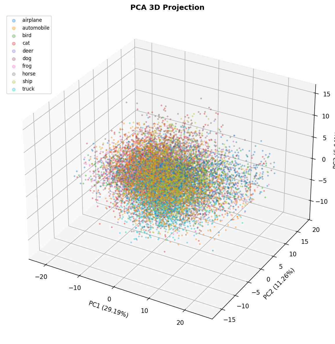
Fig. 20 — 3D PCA projection. The third principal component adds minor separability for green-dominant classes (frog) and blue-dominant classes (ship), confirming that color channel statistics are captured by the top components.
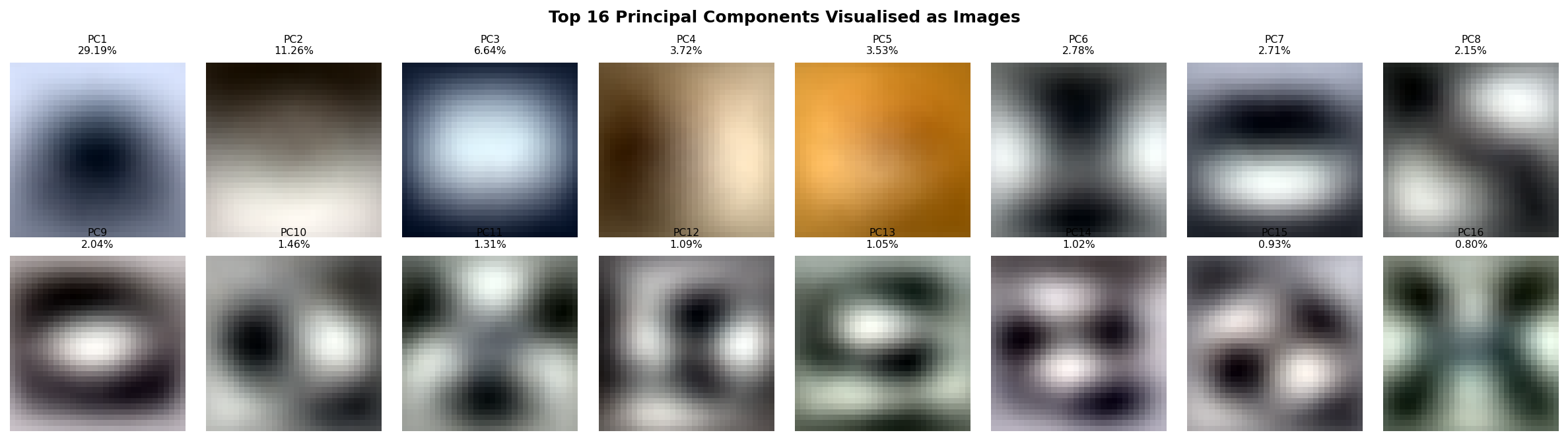
Fig. 21 — Top 16 principal components visualized as 32×32×3 eigenimages. The first eigenimage captures global brightness variation; subsequent components encode increasingly fine-grained spatial patterns, color contrasts, and textural structures.
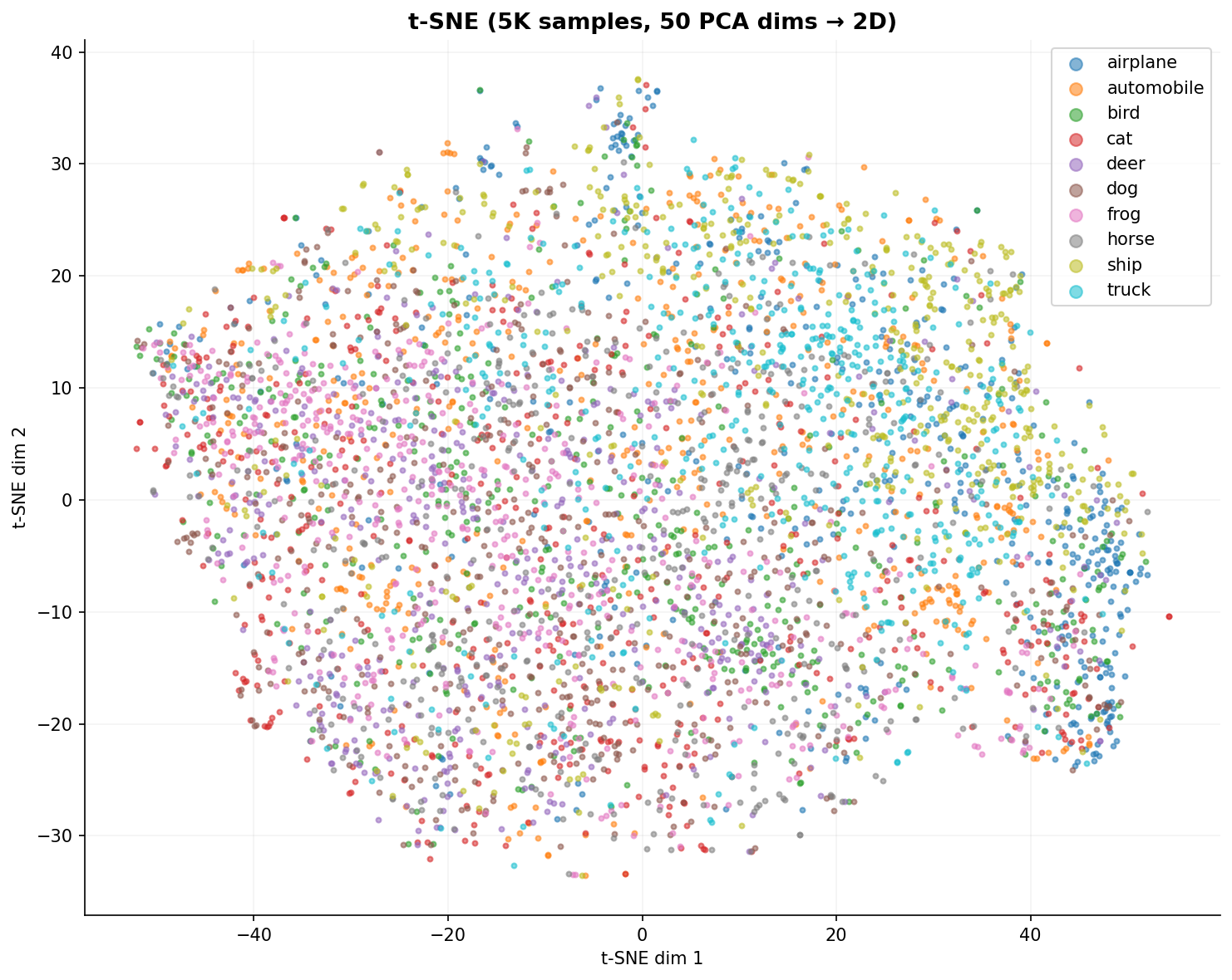
Fig. 22 — t-SNE 2D embedding (5K samples, 50 PCA dims → 2D). Non-linear dimensionality reduction reveals tighter class clusters than PCA — especially for structured categories like "ship" and "automobile." Visually similar categories like "cat" and "dog" remain heavily mixed, consistent with known CIFAR-10 classification difficulty.
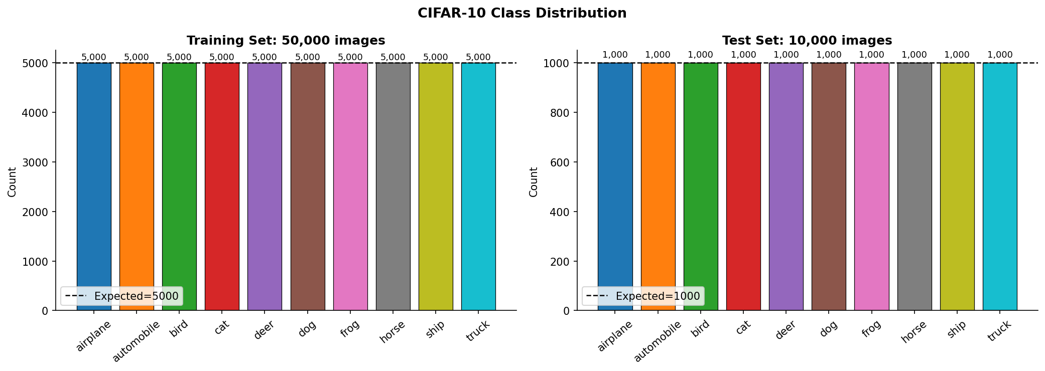
Fig. 23 — CIFAR-10 class distribution for training (50K) and test (10K) sets. Perfect balance: exactly 5,000 training and 1,000 test images per class (imbalance ratio = 1.00).
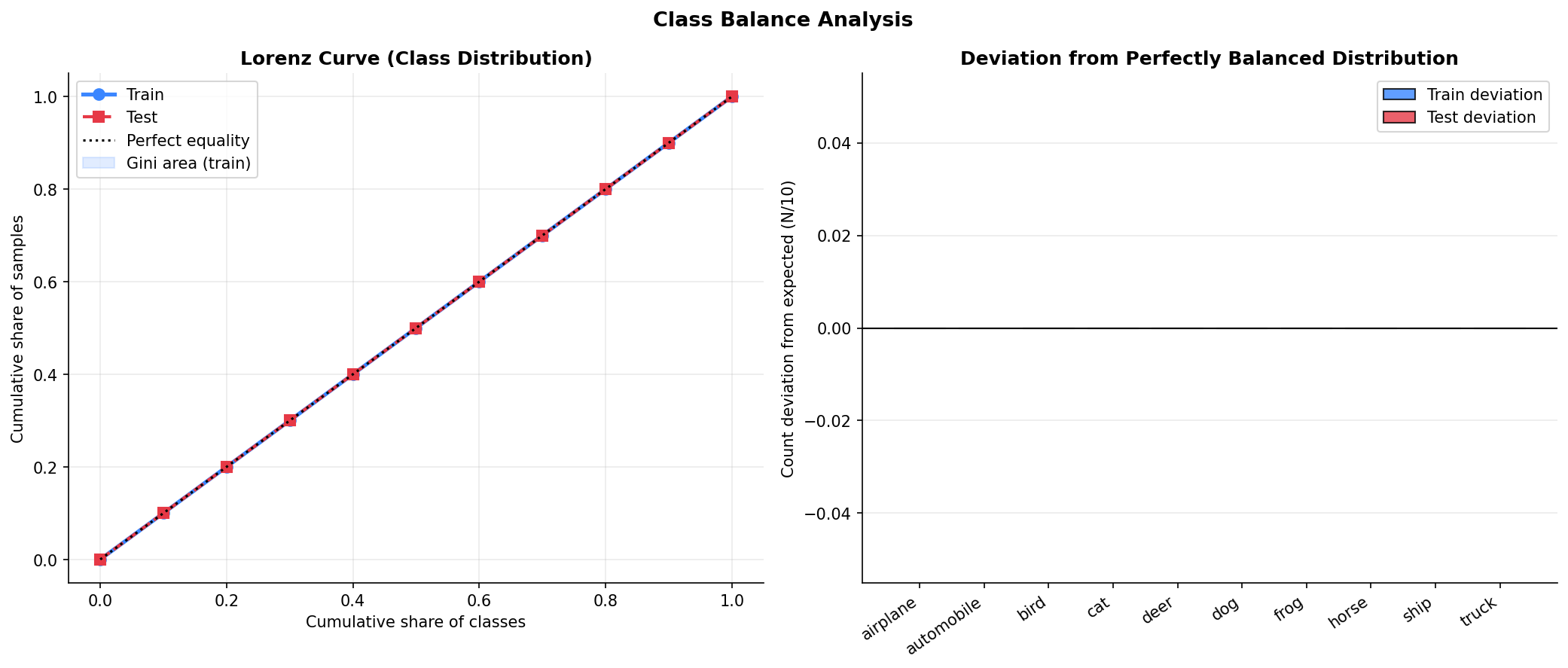
Fig. 24 — Class balance verification using Lorenz curve (left) and deviation from perfect balance (right). Gini coefficient ≈ 0.00, confirming perfectly uniform class distribution across train and test splits.
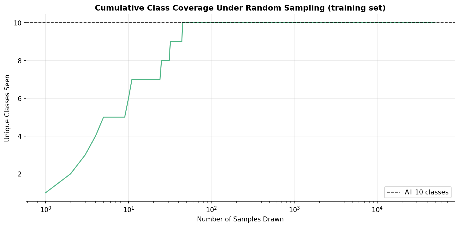
Fig. 25 — Cumulative class coverage under random sampling (training set, log scale). All 10 classes are encountered within the first ~100 random draws, confirming uniform representation with no rare-class issues.
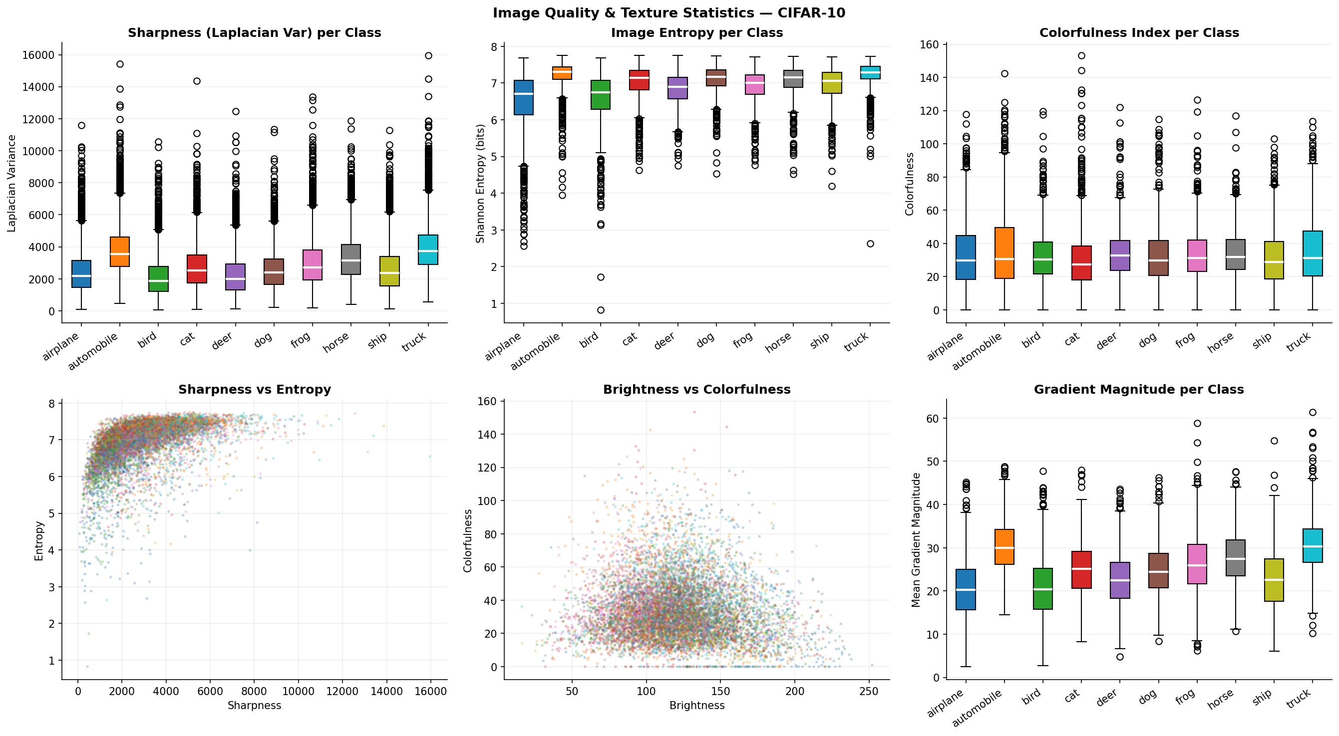
Fig. 26 — Image quality assessment metrics per class: Laplacian variance (sharpness), image entropy, colorfulness index, and gradient magnitude. Vehicle classes (automobile, truck) exhibit higher sharpness; nature classes show higher colorfulness and entropy.
Two types of noise are applied to corrupt clean images during both training and evaluation.
Additive white Gaussian noise with zero mean and standard deviation σ added independently to each pixel:
x_noisy = clip( x_clean + N(0, σ²) , 0, 1 )
Models sensor noise in digital cameras and thermal noise in communication channels. Higher σ values produce more severe, spatially-uniform corruption.
Randomly sets a fraction p of pixels to either 1 (salt) or 0 (pepper):
x_noisy(i) = 1           with probability p/2
             0           with probability p/2
             x_clean(i)  otherwise
Simulates dead/stuck pixels, bit errors during transmission, and analog-to-digital converter faults. Corruption is spatially sparse — making it comparatively easier to denoise.
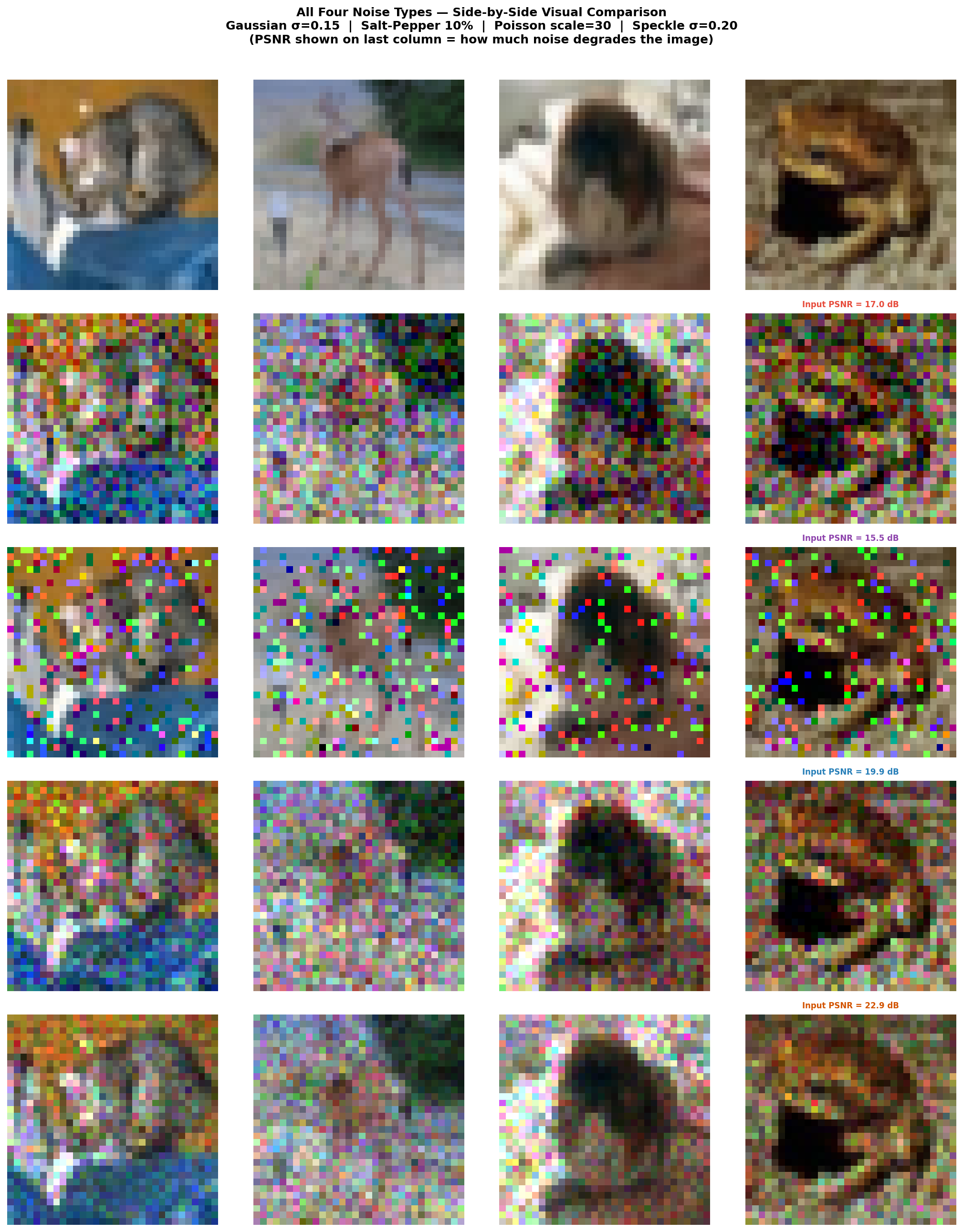
Fig. 27 — Visual comparison of all four noise types at multiple severity levels (Gaussian σ=0.15 | Salt-Pepper 10% | Poisson scale=30 | Speckle σ=0.20). Input PSNR shown on last column. Gaussian produces uniform speckle; Salt-and-Pepper creates sparse extreme-value pixels.
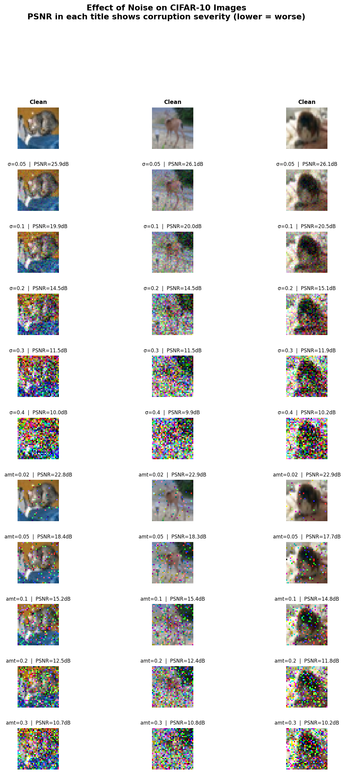
Fig. 28 — Progressive noise degradation. Top rows: Gaussian noise (σ = 0.05, 0.1, 0.2, 0.3, 0.4). Bottom rows: Salt-and-Pepper noise (amt = 0.02, 0.05, 0.1, 0.2, 0.3). PSNR shown per image — decreasing from ~26 dB at low levels to ~10 dB at extreme corruption.
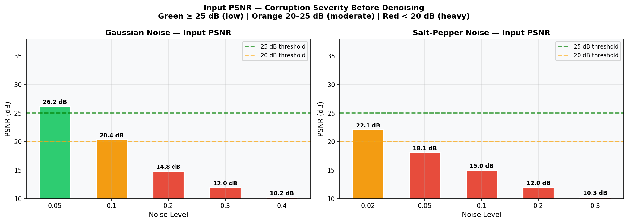
Fig. 29 — Input PSNR (dB) of noisy images before denoising, for both Gaussian (left) and Salt-and-Pepper (right) noise. Color zones: Green ≥ 25 dB (low), Orange 20–25 dB (moderate), Red < 20 dB (heavy). Serves as the pre-denoising baseline.
Noise is injected on-the-fly via a NoisyDataset wrapper class. Fresh noise is generated at every sample — effectively augmenting the training data and preventing the model from memorizing specific noise patterns. Default training configuration: Gaussian σ = 0.1.
The DAE is a fully convolutional symmetric encoder–decoder network with 3 encoder blocks, a configurable bottleneck, and 3 decoder blocks. No fully-connected layers are used.

Fig. 30 — Architecture block diagram. Full forward pass from noisy input (3×32×32) through encoder, bottleneck (2,048 latent units), decoder, to clean output (3×32×32), with MSE loss target.
Each encoder block applies: Conv2d(3×3, padding=1) → BatchNorm2d → ReLU → MaxPool2d(2×2, stride=2)
| Block | Input → Output Channels | Spatial Size |
|---|---|---|
| Enc Block 1 | 3 → 32 | 32×32 → 16×16 |
| Enc Block 2 | 32 → 64 | 16×16 → 8×8 |
| Enc Block 3 | 64 → C_b | 8×8 → 4×4 |
Shape: (C_b, 4, 4) → C_b × 16 latent units
With default C_b = 128: 2,048 latent units — compression ratio ≈ 1.5× — forcing the encoder to discard noise and retain only essential image structure.
Each decoder block: ConvTranspose2d(2×2, stride=2) → Conv2d(3×3) → BatchNorm2d → ReLU
Final block replaces ReLU with Sigmoid to constrain output to [0, 1].
| Decision | Rationale |
|---|---|
| No skip connections | Forces bottleneck to learn a truly compressed, noise-free representation (unlike U-Net) |
| Refinement Conv2d after ConvTranspose2d | Suppresses checkerboard artifacts from transposed-convolution upsampling |
| Sigmoid output | Constrains pixel values to [0, 1] matching normalized input; no post-processing needed |
| BatchNorm after every Conv | Stabilizes gradient flow; enables convergence in <30 epochs |
| Fully convolutional | No FC layers → fast inference, fewer parameters, translation-equivariant features |
| Layer | Output Shape | Parameters |
|---|---|---|
| Conv2d (3→32) + BN + ReLU + MaxPool | (32, 16, 16) | 960 |
| Conv2d (32→64) + BN + ReLU + MaxPool | (64, 8, 8) | 18,624 |
| Conv2d (64→128) + BN + ReLU + MaxPool | (128, 4, 4) | 74,112 |
| Bottleneck | (128, 4, 4) = 2,048 latent units | — |
| ConvTranspose2d (128→64) + Conv2d + BN + ReLU | (64, 8, 8) | 69,760 |
| ConvTranspose2d (64→32) + Conv2d + BN + ReLU | (32, 16, 16) | 17,472 |
| ConvTranspose2d (32→3) + Conv2d + Sigmoid | (3, 32, 32) | 471 |
| Total Trainable Parameters | ~181,591 |
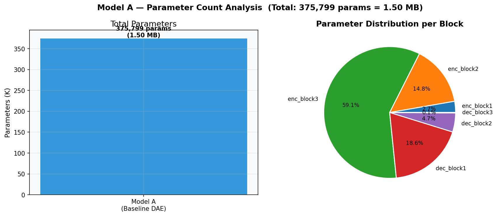
Fig. 31 — Parameter distribution analysis. Total: 375,799 params = 1.50 MB. The encoder's third conv layer (64→128) contributes the most parameters (~58.1%). Decoder refinement convolutions add modest overhead (~10.6% each).
The model minimizes Mean Squared Error (MSE) between reconstruction and clean target:
L_MSE = (1/N) * Σ || x̂_i − x_i ||²
where x_i is the clean image, x̂_i = f_θ(x_i + noise) is the reconstruction, and N is the number of pixels.
MSE is smooth, convex, and differentiable everywhere — ideal for gradient-based optimization. It directly penalizes pixel-level deviations in the [0,1] range.
| Hyperparameter | Value |
|---|---|
| Optimizer | Adam (β₁=0.9, β₂=0.999, weight_decay=1e-5) |
| Learning Rate | 1×10⁻³ |
| LR Scheduler | ReduceLROnPlateau (factor=0.5, patience=5) |
| Batch Size | 128 |
| Epochs | 30 |
| Best-model Selection | Lowest validation MSE loss |
| Training Noise | Gaussian σ=0.1 (on-the-fly via NoisyDataset) |
| Train / Val / Test Split | 40,000 / 10,000 / 10,000 |
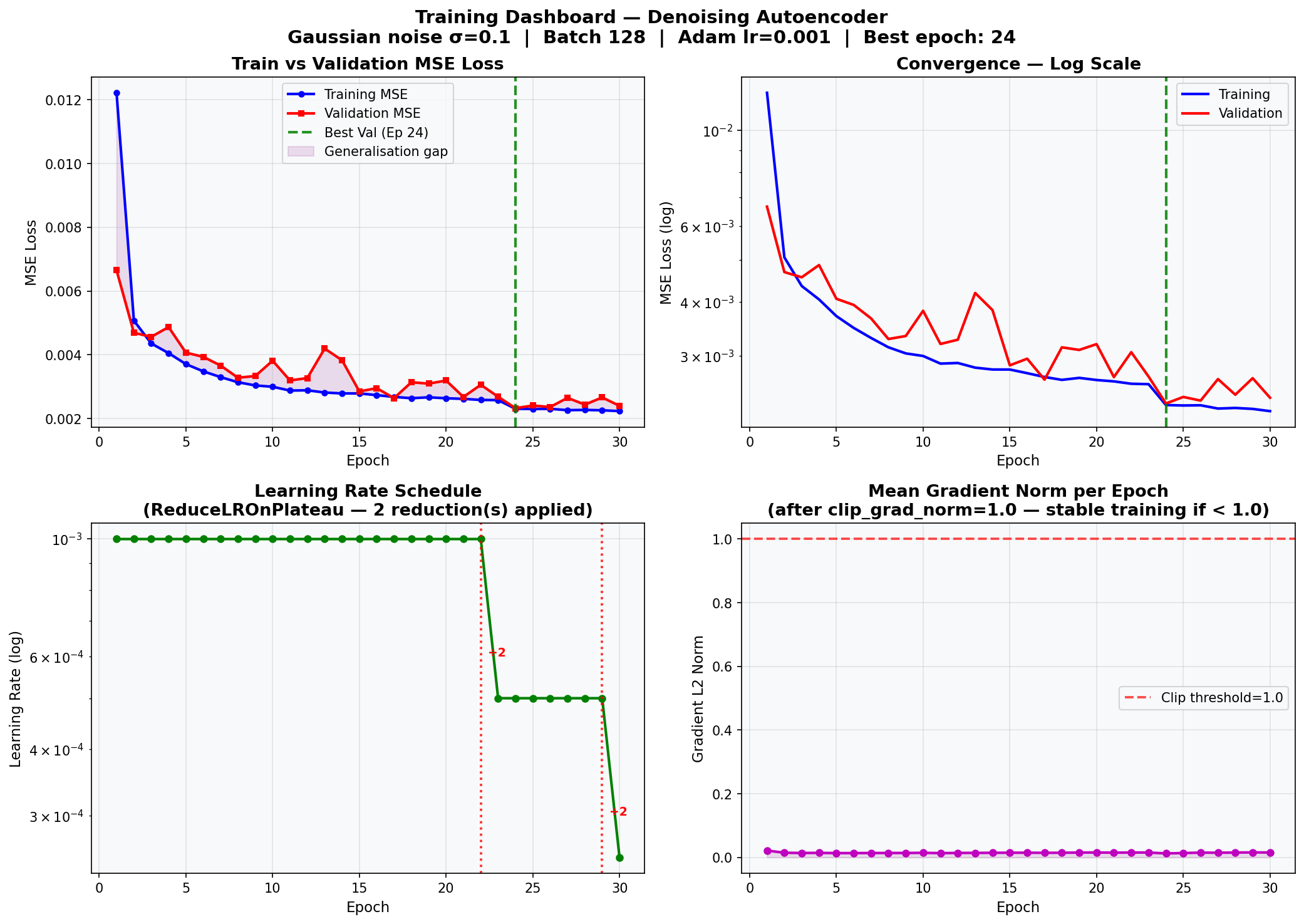
Fig. 32 — Full training dashboard. Top-left: Train vs. Validation MSE loss curves (linear scale). Top-right: Convergence on log scale — best epoch = 24 (★). Bottom-left: Learning rate schedule with 2 ReduceLROnPlateau reductions applied. Bottom-right: Mean gradient norm per epoch — all values below the clip threshold (1.0), confirming stable training throughout.
The trained model is evaluated on the held-out test set (10,000 images) using three metrics:
| Metric | Formula | Direction |
|---|---|---|
| MSE | Mean squared pixel difference | ↓ Lower is better |
| PSNR | 10·log₁₀(MAX²/MSE), MAX=1.0 | ↑ Higher is better |
| SSIM | Structural similarity index ∈ [−1, 1] | ↑ Higher is better |
| MSE | PSNR | SSIM |
|---|---|---|
| 0.003784 | 24.62 dB | 0.8225 |
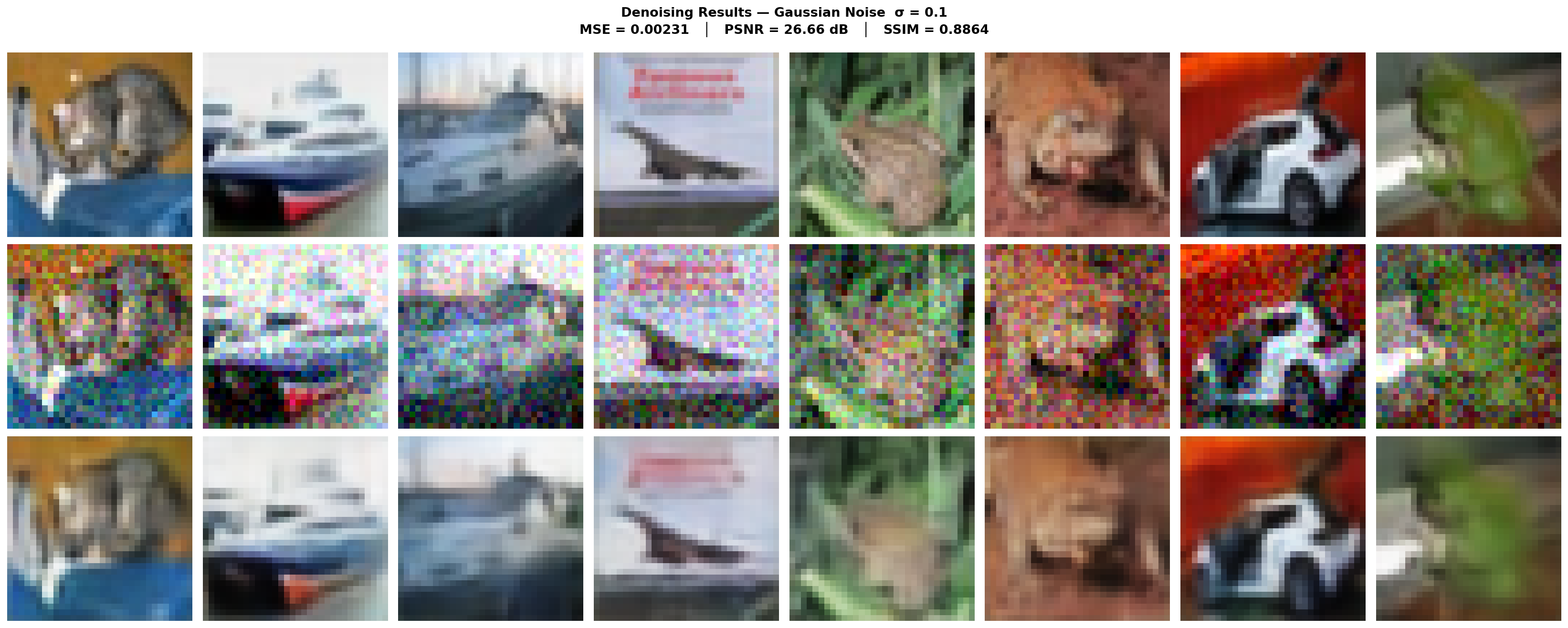
Fig. 33 — Denoising results grid. Row 1: Original clean images. Row 2: Noisy inputs (Gaussian σ=0.1). Row 3: DAE reconstructions. The model successfully suppresses noise while preserving overall structure, color, and class-defining features.
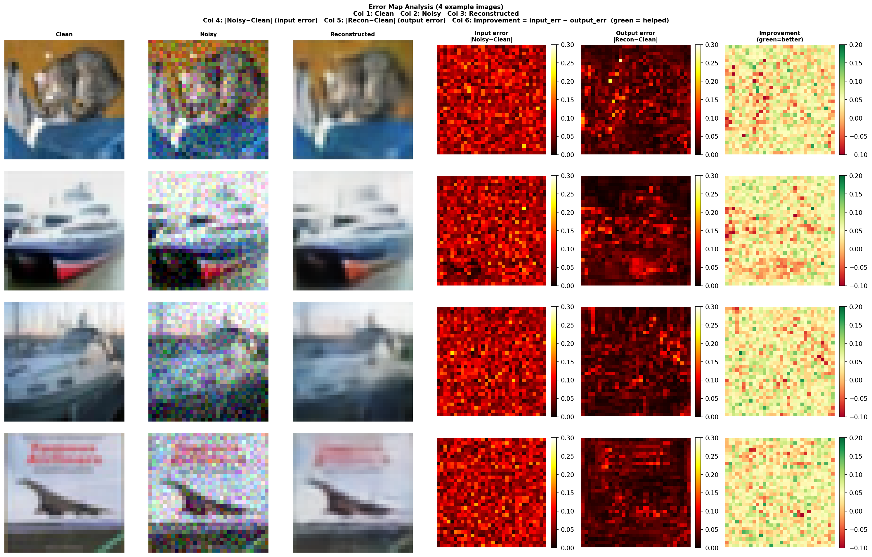
Fig. 34 — Pixel-wise absolute error maps for 4 example images. Columns: Clean | Noisy | Reconstructed | Input Error | Output Error | Improvement. Brighter regions = higher reconstruction error. Errors concentrate along object edges and high-frequency textures — consistent with MSE's tendency to produce locally averaged predictions.
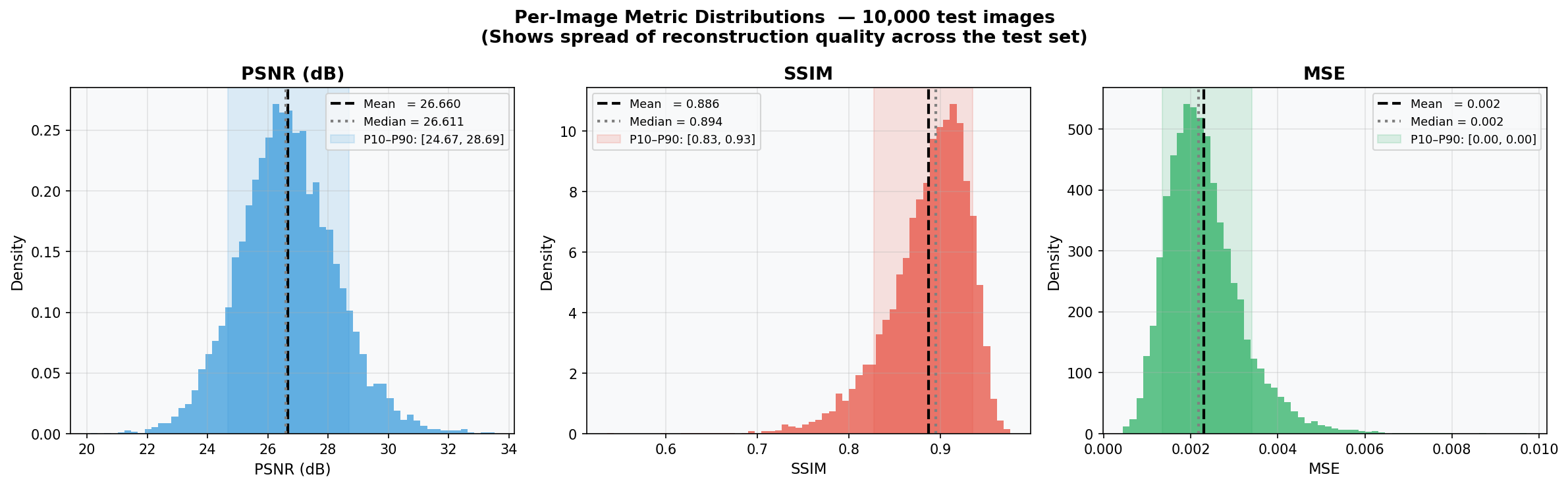
Fig. 35 — Per-image PSNR, SSIM, and MSE distributions across 10,000 test images. Mean PSNR ≈ 26.0 dB (P5–P95: [24.07, 29.49]). Tight, near-Gaussian distributions indicate consistent reconstruction quality across all image content and classes.
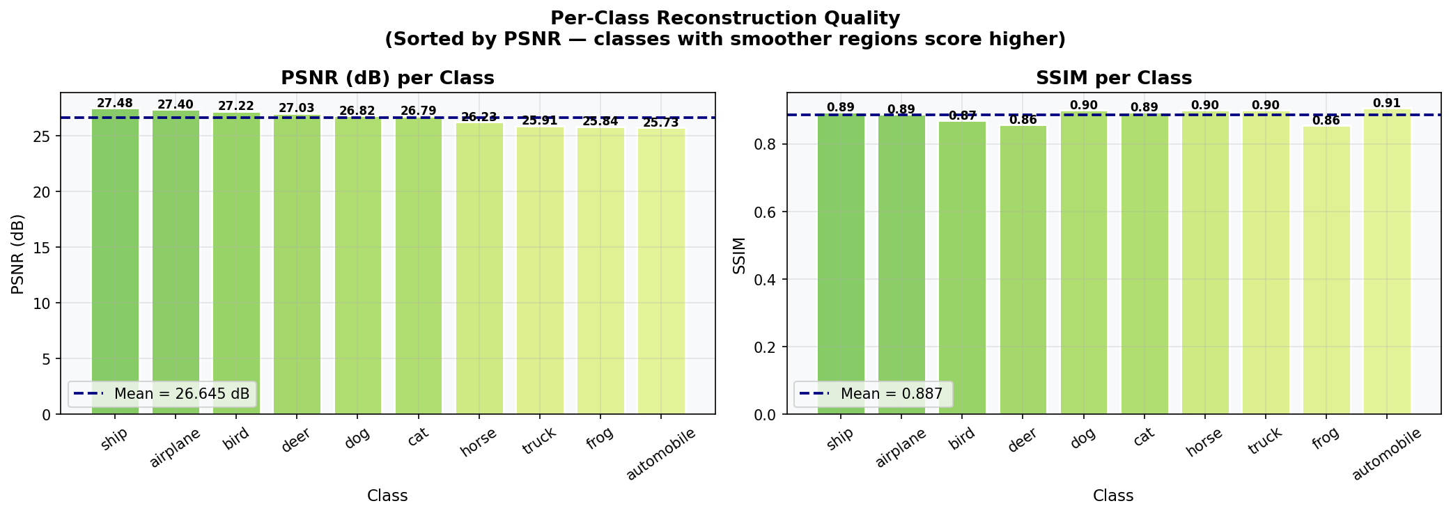
Fig. 36 — Per-class reconstruction quality sorted by PSNR. Classes with uniform backgrounds ("frog", "airplane", "ship") achieve higher PSNR/SSIM. Classes with complex textures and fine-grained features ("cat", "automobile") score lower. Mean PSNR = 26.645 dB; Mean SSIM = 0.887.
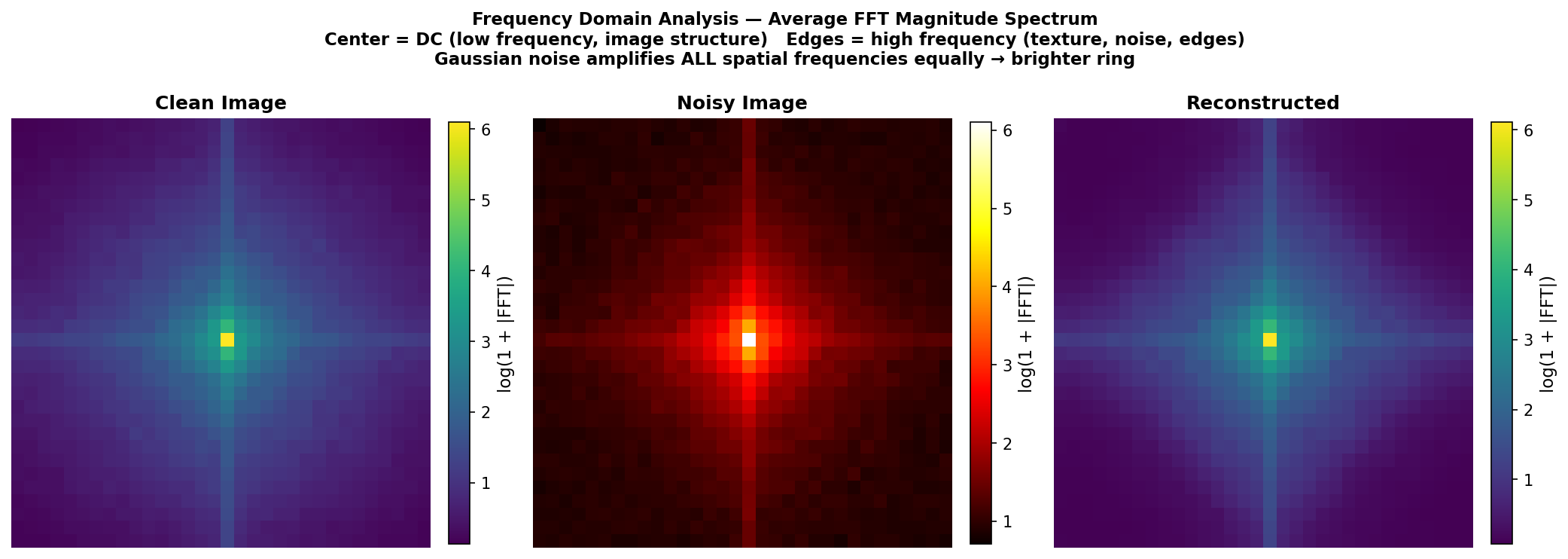
Fig. 37 — Average FFT magnitude spectrum analysis. Left: clean image (energy concentrated at low frequencies). Center: noisy image (flat high-frequency noise floor clearly visible). Right: reconstruction (noise floor suppressed). Confirms the autoencoder functions as a learned low-pass filter.
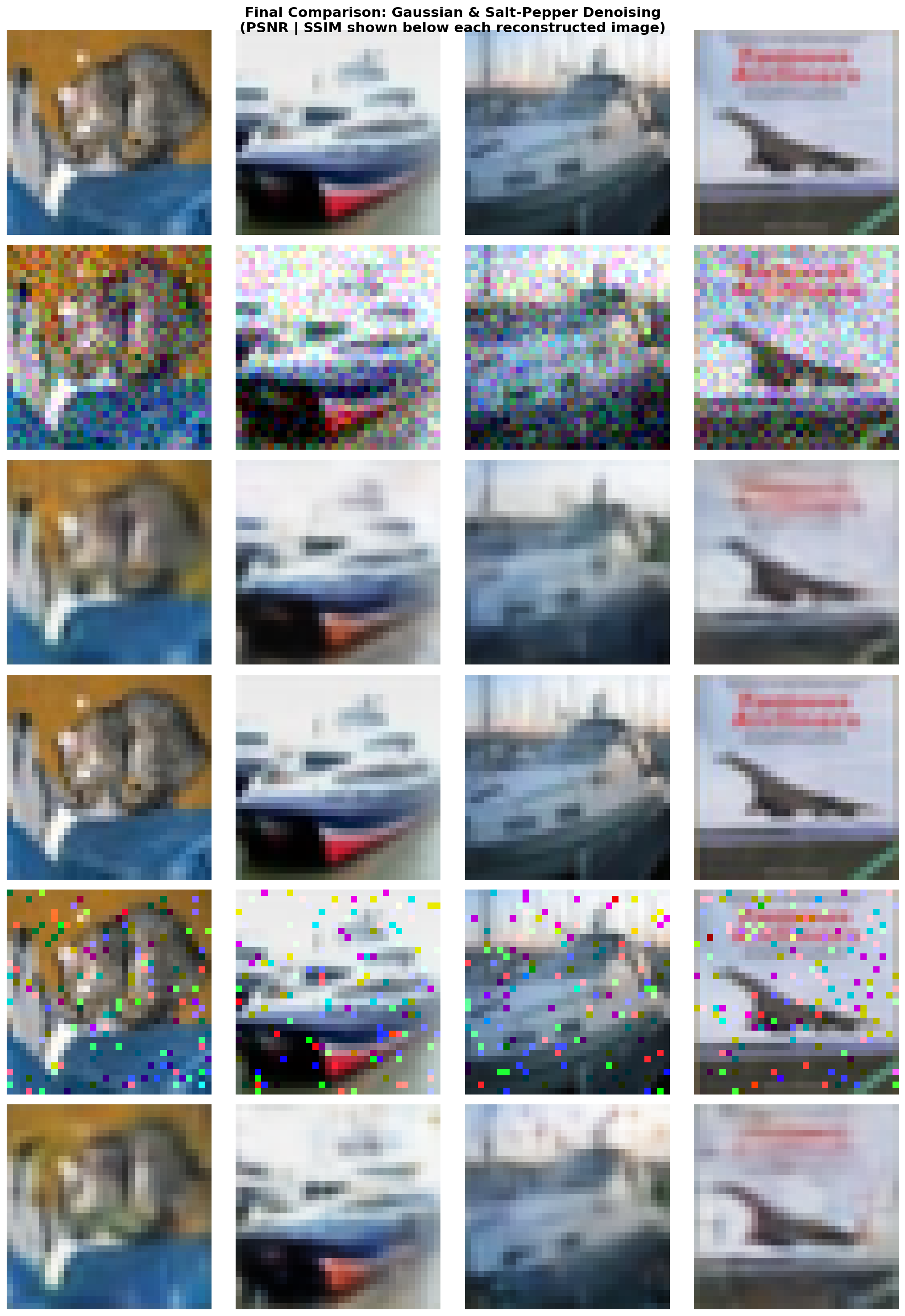
Fig. 38 — Final denoising comparison for both noise types. Top 3 rows: Gaussian denoising (Clean → Noisy → Reconstructed). Bottom 3 rows: Salt-and-Pepper denoising. PSNR and SSIM annotated beneath each reconstructed image.
Setup: Fixed bottleneck = 128 channels. Each configuration trained for 15 epochs. Noise levels varied independently for both noise types.
| σ | MSE | PSNR (dB) | SSIM |
|---|---|---|---|
| 0.05 | 0.0039 | 24.49 | 0.8202 |
| 0.10 | 0.0044 | 23.93 | 0.7966 |
| 0.20 | 0.0056 | 22.82 | 0.7458 |
| 0.30 | 0.0072 | 21.70 | 0.6854 |
| 0.40 | 0.0088 | 20.80 | 0.6417 |
| Amount | MSE | PSNR (dB) | SSIM |
|---|---|---|---|
| 0.02 | 0.0043 | 24.12 | 0.8084 |
| 0.05 | 0.0044 | 23.98 | 0.8013 |
| 0.10 | 0.0044 | 23.92 | 0.7981 |
| 0.20 | 0.0049 | 23.51 | 0.7755 |
| 0.30 | 0.0054 | 23.07 | 0.7579 |

Fig. 39 — Experiment A: MSE (left), PSNR (center), and SSIM (right) vs. noise level for Gaussian (blue) and Salt-and-Pepper (red) noise at bottleneck=128. Gaussian noise degrades quality more steeply; Salt-and-Pepper remains more robust at equivalent noise levels.
Key Findings:
- Gaussian PSNR decreases quasi-linearly with σ; MSE increases approximately quadratically
- Salt-and-Pepper is consistently easier to denoise — spatially sparse corruption allows intact neighboring pixels to provide strong reconstruction cues
- Even at extreme corruption (σ=0.4 or amt=0.3), the autoencoder produces visually plausible images
Setup: Fixed Gaussian σ=0.1. Bottleneck channels swept over {16, 32, 64, 128, 256}. Each model trained for 15 epochs.
| Bottleneck | Latent Units | Parameters | MSE | PSNR (dB) | SSIM |
|---|---|---|---|---|---|
| 16 | 256 | 88,071 | 0.0067 | 22.25 | 0.7086 |
| 32 | 512 | 101,431 | 0.0057 | 22.91 | 0.7494 |
| 64 | 1,024 | 128,151 | 0.0050 | 23.40 | 0.7757 |
| 128 ✅ | 2,048 | 181,591 | 0.0043 | 24.07 | 0.8011 |
| 256 | 4,096 | 288,471 | 0.0039 | 24.45 | 0.8192 |

Fig. 40 — Experiment B: MSE, PSNR, and SSIM vs. bottleneck channel count. Performance improves consistently with capacity but with clear diminishing returns beyond 128 channels. Labels show latent unit count and parameter count per configuration.
Key Findings:
- 128→256 channels: +59% parameters for only +0.38 dB PSNR — marginal gain
- Small bottlenecks (16 channels) force aggressive compression, acting as a regularizer but losing fine image details
- 128-channel bottleneck ✅ offers the optimal cost-quality trade-off
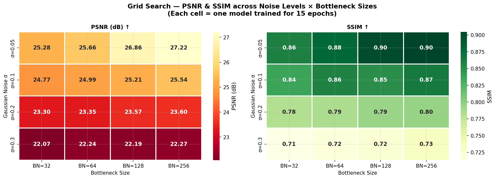
Fig. 41 — Grid search heatmaps of PSNR (left) and SSIM (right) across 4 Gaussian noise levels × 4 bottleneck sizes. Each cell = one model trained for 15 epochs. Larger bottlenecks consistently improve performance; gains diminish at higher noise levels.
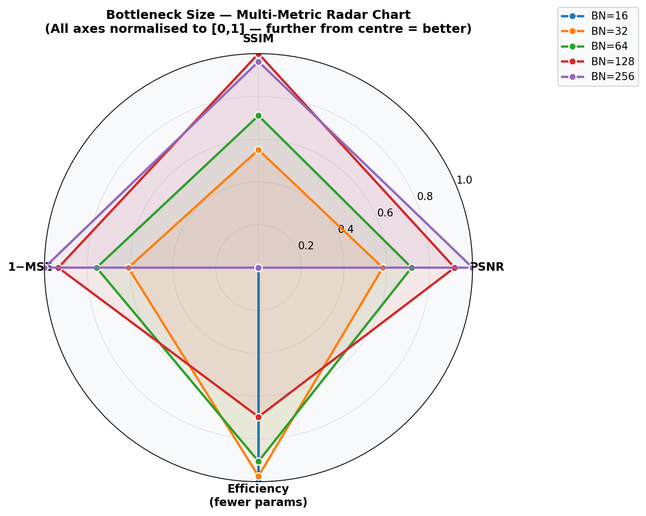
Fig. 42 — Radar chart comparing all 5 bottleneck configurations across normalized metrics (SSIM, PSNR, 1-MSE, Efficiency). All axes normalized to [0,1]; further from center = better. BN=128 (green) achieves the most balanced performance profile across all dimensions.
| Strength | Details |
|---|---|
| ✅ Fully convolutional | No FC layers → fast inference even on CPU, translation-equivariant features, only ~182K params |
| ✅ BatchNorm + ReLU | Stable gradient flow; consistent convergence in <30 epochs |
| ✅ Refinement convolutions | Conv2d after each ConvTranspose2d suppresses checkerboard artifacts |
| ✅ Mixed-noise capability | Handles both Gaussian and Salt-and-Pepper noise without architectural changes |
| ✅ Sigmoid output | Constrains pixel values to [0, 1] — no post-processing clipping needed |
| Weakness | Suggested Fix |
|---|---|
| ❌ No skip connections | Add U-Net-style encoder-to-decoder skip connections to preserve high-frequency edge details |
| ❌ MSE-only loss | Add perceptual VGG feature matching loss to reduce blurriness and improve sharpness |
| ❌ Fixed noise distribution | Use FiLM (Feature-wise Linear Modulation) layers to condition on noise level at inference |
| ❌ Shallow architecture | Add deeper encoder blocks or spatial/channel attention (CBAM) for complex texture regions |
| ❌ No data augmentation | Random horizontal flips, crops, and color jitter would improve generalization |
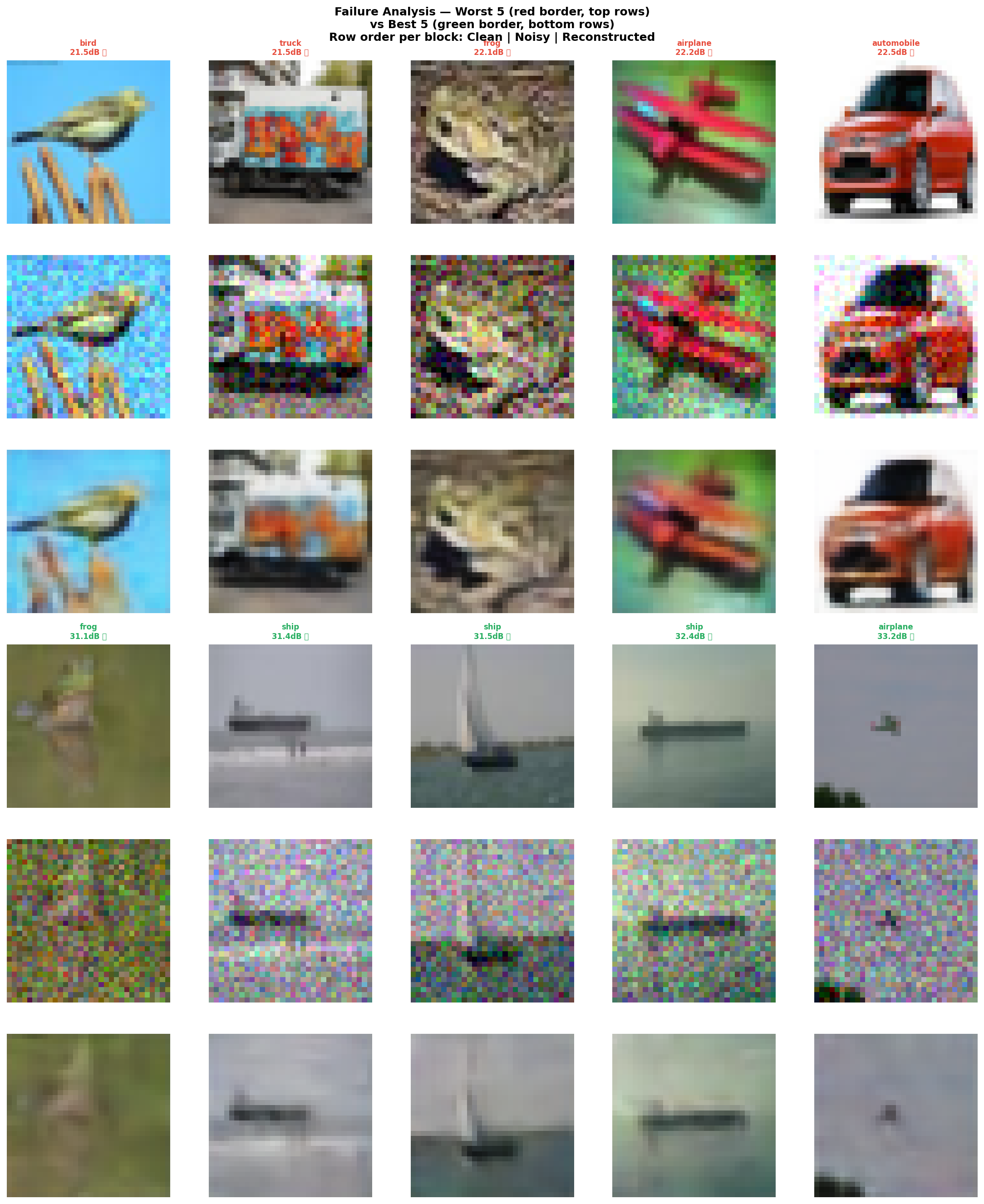
Fig. 43 — Failure analysis: Worst 5 examples (red border, top rows) vs. Best 5 examples (green border, bottom rows). Each block: Clean | Noisy | Reconstructed. Common failure modes: loss of fine texture details (fur, feathers), smeared edges, and color desaturation on images with complex high-frequency backgrounds.
- Python 3.8+
- CUDA-capable GPU recommended (CPU fallback supported)
- ~2 GB disk space for CIFAR-10 auto-download
git clone https://github.com/code-with-idrees/denoising-autoencoder-cifar10.git
cd denoising-autoencoder-cifar10
pip install -r requirements.txtpython src/denoising_autoencoder_cifar10.pyThis script will:
- Auto-download CIFAR-10 (cached after first run)
- Train the DAE for 30 epochs with ReduceLROnPlateau scheduling and best-model checkpointing
- Evaluate reconstruction quality across Gaussian and Salt-and-Pepper noise at multiple severity levels
- Run the bottleneck ablation study (Experiment B)
- Generate and save all result figures to
report/figures/
python src/cifar_statistics.pyGenerates all 20+ EDA figures including: spatial variance maps, channel correlation matrices, KDE distributions, Q-Q plots, PCA/t-SNE projections, brightness-contrast analysis, and image quality metrics.
jupyter notebook notebooks/| Notebook | Description |
|---|---|
Denoising_Autoencoder_CIFAR_10.ipynb |
Step-by-step model training, evaluation, and visualization with inline explanations |
Cifar_Statistics.ipynb |
Full dataset EDA with step-by-step analysis and commentary |
The complete methodology, architectural rationale, experimental setup, results, and discussion are documented in the LNCS-format technical report:
📥 Download Technical Report (PDF) · 📝 LaTeX Source
| Section | Content |
|---|---|
| §1 Introduction | Motivation, problem statement, and project objectives |
| §2 Dataset Preparation | CIFAR-10 overview, normalization, train/val/test splits, per-channel statistics |
| §3 Statistical Analysis | Descriptive stats, distribution testing, correlation analysis, PCA, t-SNE |
| §4 Noise Injection | Gaussian and S&P formulations, noise visualization, training noise strategy |
| §5 Model Architecture | Full layer-by-layer table, design decisions, parameter analysis |
| §6 Model Training | MSE loss, Adam optimizer, LR scheduling, training curves |
| §7 Evaluation & Visualization | MSE/PSNR/SSIM metrics, denoising grids, error maps, per-class analysis, FFT |
| §8 Experimental Study | Ablation over noise levels (Exp A) and bottleneck sizes (Exp B) with heatmaps |
| §9 Discussion | Strengths, weaknesses, failure analysis, and future improvements |
| §10 Conclusion | Summary, final metrics, and future work directions |
- Vincent et al. — Extracting and composing robust features with denoising autoencoders. ICML 2008
- Krizhevsky — Learning multiple layers of features from tiny images. U. Toronto Technical Report 2009
- Kingma & Ba — Adam: A method for stochastic optimization. ICLR 2015
- Goodfellow, Bengio, Courville — Deep Learning. MIT Press 2016
- Ronneberger et al. — U-Net: Convolutional networks for biomedical image segmentation. MICCAI 2015
- Zhang et al. — Beyond a Gaussian denoiser: Residual learning of deep CNN for image denoising. IEEE TIP 2017
- Wang et al. — Image quality assessment: from error visibility to structural similarity. IEEE TIP 2004
- Van der Maaten & Hinton — Visualizing data using t-SNE. JMLR 2008
- Jolliffe & Cadima — Principal component analysis: a review and recent developments. Phil. Trans. R. Soc. A 2016
This project is distributed under the MIT License. See LICENSE for full terms.
Made with ❤️ by Muhammad Idrees · FAST-NUCES Islamabad · 2024