FitPDF fits complex mixture models of various distributions to observational data. This is useful, for instance, for characterising the observed pulse energy distributions of radio pulsars and repeating fast radio bursts (FRBs). However, FitPDF is data-agnostic and can, in principle, fit any distribution data and determine its underlying probability density function (PDF).
The FitPDF software suite includes tools for simulating distribution data, fitting complex mixture distributions to data, and comparing the resulting fits in an information-theoretical sense. FitPDF support several model distributions, which are homogeneous or heterogeneous mixtures of individual component distributions (e.g. normal, lognormal, power law). FitPDF operates in a Bayesian and unbinned manner, thereby maximising the information extracted from the data and robustly determining the model parameters and their uncertainties.
The current implementation is based on PyMC.
The software is primarily developed and maintained by Fabian Jankowski. For more information, feel free to contact me via: fabian.jankowski at cnrs-orleans.fr.
The corresponding paper is currently in preparation.
If you make use of the software, please add a link to this repository and cite our corresponding paper. See above and the CITATION and CITATION.bib files.
The easiest and recommended way to install the software is via the Python command pip directly from the FitPDF GitHub software repository. For instance, to install the master branch of the code, use the following command:
pip install git+https://github.com/fjankowsk/fitpdf.git@master
This will automatically install all dependencies. Depending on your Python installation, you might want to replace pip with pip3 in the above command.
The latest stable version of the code should also be available on the Python package index PyPI.
$ fitpdf-compare -h
usage: fitpdf-compare [-h] [-o] files [files ...]

Compare fits.

positional arguments:
  files         Names of files to process. The input files must be InferenceData files produced by fitpdf-fit.

options:
  -h, --help    show this help message and exit

Output formatting:
  -o, --output  Output plots to file rather than to screen. (default: False)
$ fitpdf-fit -h
usage: fitpdf-fit [-h] [--mean value] [--fast] [--model {NL,NN,NNL,NNP}] [--weights value [value ...]] [--label name] [--nbin value] [-o] [--publish] [--title text] filename
Fit distribution data.
positional arguments:
filename Name of file to process. The input file must be produced by the fluence time series option of plot-profilestack.
options:
-h, --help show this help message and exit
--mean value The global mean fluence by which to divide the histograms. The default behaviour is to determine it automatically from the on-pulse fluence data. (default: None)
Fit parameters:
--fast Enable fast processing. This reduces the number of MCMC samples drastically and is recommended against for publication-quality fits. (default: False)
--model {NL,NN,NNL,NNP}
Use the specified distribution model, where N denotes a Normal, L a Lognormal, and P a powerlaw (Pareto) component. For instance, the default NNL model consists of two Normal and one Lognormal distributions. (default: NNL)
--weights value [value ...]
Override the default component distribution weights in the model prior. This is sometimes useful to ensure convergence of the fit. The weights are given as simple floating point numbers (not percentages) and must sum to unity. For instance,
[0.2, 0.3, 0.5] assigns an average prior weight of 20, 30, and 50 per cent to each of the component distributions, respectively. The number of weights specified must match the number of model components, e.g. three for the NNL model. (default:
None)
Output formatting:
--label name The label to use for the input file. (default: None)
--nbin value The number of histogram bins to use. (default: 50)
-o, --output Output plots to file rather than to screen. (default: False)
--publish Produce plots suitable for publication. (default: False)
--title text Set a custom figure title. (default: None)$ fitpdf-simulate -h
usage: fitpdf-simulate [-h] [--nsamp value] [--randomseed value] [-o]
Simulate distributions.
options:
-h, --help show this help message and exit
--nsamp value Number of random samples to draw from the simulated distribution. (default: 10000)
--randomseed value Enable deterministic mode by providing a seed value for the random number generator. This is useful if you want to fix the underlying distribution when changing the
number of samples. The default behaviour is non-deterministic, i.e. the simulation uses different distribution parameters in each run. (default: None)
Output formatting:
-o, --output Output plots to file rather than to screen. (default: False)FitPDF reads the input distribution data from simple plain text files in comma-separated values (CSV) format. The files must contain at least the following data fields or columns:
- "rotation": integer
The rotation or pulse number corresponding to the fluence entry.
- "zapped": boolean or integer (True/False or 0/1)
A flag indicating whether the rotation has been zapped or RFI excised. All entries where zapped == True are excluded from the fitting.
- "fluence_on": float
The fluence or flux density integrated (summed) across the on-pulse phase range.
- "nbin_on": integer
The width of the on-pulse phase range in bins.
- "fluence_off": float
The fluence or flux density integrated (summed) across the entire off-pulse phase range.
- "nbin_off": integer
The width of the off-pulse phase range in bins.
- "fluence_off_same": float
The fluence or flux density integrated (summed) across a subset of the off-pulse phase range of the same width as the on-pulse window.
- "nbin_off_same": integer
The width of the off-pulse phase range subset in bins.
The line below provides a minimal CSV header that you can use.
rotation,zapped,fluence_on,nbin_on,fluence_off,nbin_off,fluence_off_same,nbin_off_same
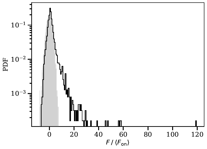
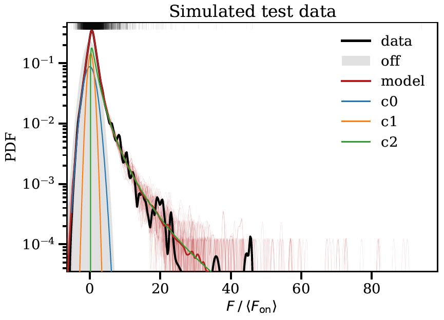
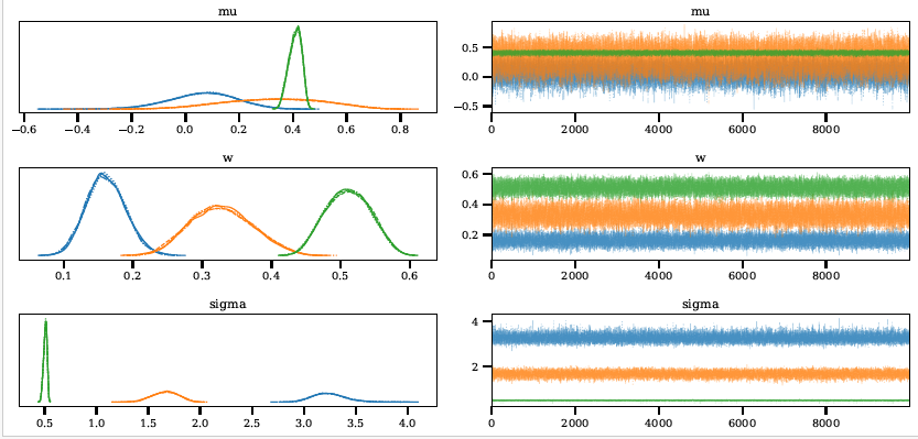
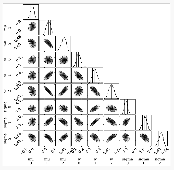
The images below show some example output from the program obtained when fitting simulated test data.


