
This project addressed a traffic sign classification problem using deep learning models. To achieve this I considered two feed forward convolutional neural network architectures implemented in python using google's Tensorflow framework via the python API. I use the the German Traffic Sign Recognition Benchmark (GTSRB) data set to train and test the deep learning models. Once satisfactory performance had been achieved on the GTSRB data set, I then applied the models to real traffic signs on German roads acquired though google maps. The classification performance of the models is then evaluated.
This work was done as part of the Udacity Self Driving Car Nano-Degree program
Historical development of road infrastructure has been done with the human visual system being the key method of information transfer between the environment and vehicle by means of a human perception and then control. Any autonomous driving system capable of safely operating in existing road environments must then as a bare minimum be capable of human level visual recognition of the environment it operates in. Visual classification is a key element within more complex visual recognition tasks (such as object detection and semantic segmentation) and also a key task in the visual perception of an autonomous vehicle for correct classification of road signs.
The German Traffic Sign Recognition Benchmark (GTSRB) data set is a multi-class, single-image classification challenge made up of images of traffic signs taken from German roads, with an associated class label for each image in the dataset. The images are extracted from video data of an on-board a moving car camera removing all temporal information.
The size of the data-set is summarised as follows
-
Each image is 32 x 32 pixels made up of 3 colour channels formatted in RGB. Each pixel is saved using an 8 bit unsigned integer giving a total of 256 possible values.
-
Each image belongs to one of 43 unique classes/labels grouped by the design/meaning of the sign.
-
The training set is made up of 34799 images with their associated labels.
-
The validation set is made up of 4410 images with their associated labels.
-
The test set is made up of 12630 images with their associated labels
The data set can be downloaded here.
On initial thought, correctly classifying traffic signs could be considered to be a fairly simple task due to the design of traffic signs being unique and showing extremely little variably in apprentice within each class. In addition to this, the designs are typically simple and are placed in positions which should be clear to drivers to identify. However there are many aspects of the GTSRB data set that is challenging from the point of view of accurate classification, these include
- Variations in viewpoint
- Variation in brightness of lighting condition
- Motion blur (due to the video capture)
- Damages to signs
Many of these artefacts can be seen by viewing the images from the dataset below

The random sample above is typical of the dataset as a whole. Variation in the brightness of each sample is typically the most notable visual degradation and should be given attention in the preprocessing stage.
A histogram plot of the number of each samples per class shows a large imbalance in distribution across the classes. Some classes contain as many as almost 10 times the number of samples as others. This imbalance in distribution should be addressed to prevent any bias arising in training the model on this dataset.

Observing the GTSRB data sets two things became very apparent
-
The dataset has a large imbalance in the number of sample occurrences across classes. That is to say some classes contain a lot more image data samples then others.
-
The size of the data set is insufficient for training a high capacity deep network, and over-fitting to this small training set is likely to occur.
To address both of these issues, I used data augmentation techniques to create new image samples, artificially enlarging the data set using class preserving image transformations. The images were generated in such way that the resulting augmented training distribution was balanced across classes.
The data augmentation pipeline is made up of three components that will be used in series applying randomly generated parameters to generate the transformations. The transforms used are chosen so that once applied the underlying class content is maintained. For example, mirror flipping a left turn sign would make it a right turn and should not be used. The transformations were chosen to be typical of the types of distortions the classifier should be robust to. The following three components make up the pipeline
I first apply a rotation of a random angle between -15 and +15 degrees to the input image
from skimage.transform import rotate

def rotate_image(image, max_angle =15):
    rotate_out = rotate(image, np.random.uniform(-max_angle, max_angle), mode='edge')
    return rotate_out
Next I apply a random translation in the height and width up-to a maximum translation of 5 pixels.
import cv2

def translate_image(image, max_trans = 5, height=32, width=32):
    translate_x = max_trans*np.random.uniform() - max_trans/2
    translate_y = max_trans*np.random.uniform() - max_trans/2
    translation_mat = np.float32([[1,0,translate_x],[0,1,translate_y]])
    trans = cv2.warpAffine(image, translation_mat, (height,width))
return trans![]()
Finally I apply a projection (homography) transform with randomly selected co-ordinates
from skimage.transform import ProjectiveTransfor

def projection_transform(image, max_warp=0.8, height=32, width=32):
    #Warp Location
    d = height * 0.3 * np.random.uniform(0,max_warp)

    #Warp co-ordinates
    tl_top = np.random.uniform(-d, d)     # Top left corner, top margin
    tl_left = np.random.uniform(-d, d)    # Top left corner, left margin
    bl_bottom = np.random.uniform(-d, d)  # Bottom left corner, bottom margin
    bl_left = np.random.uniform(-d, d)    # Bottom left corner, left margin
    tr_top = np.random.uniform(-d, d)     # Top right corner, top margin
    tr_right = np.random.uniform(-d, d)   # Top right corner, right margin
    br_bottom = np.random.uniform(-d, d)  # Bottom right corner, bottom margin
    br_right = np.random.uniform(-d, d)   # Bottom right corner, right margin

    ##Apply Projection
    transform = ProjectiveTransform()
    transform.estimate(np.array((
                (tl_left, tl_top),
                (bl_left, height - bl_bottom),
                (height - br_right, height - br_bottom),
                (height - tr_right, tr_top)
            )), np.array((
                (0, 0),
                (0, height),
                (height, height),
                (height, 0)
            )))
    output_image = warp(image, transform, output_shape=(height, width), order = 1, mode = 'edge')
    return output_image
Using these three transforms gives the full class preserving data augmentation pipeline. Examples of typical images produced using this pipeline are shown below.


The augmentation pipeline was applied to images in the training set until each class contained 10000 training examples. This was done to create a new augmented training data set containing 430000 samples in total.
Observation of the data set showed a large amount of variation in brightness across images in the data set. To remove this the first pre-processing technique was to normalise the brightness across image channels.
import cv2

def image_brightness_normalisation(image):
    image[:,:,0] = cv2.equalizeHist(image[:,:,0])
    image[:,:,1] = cv2.equalizeHist(image[:,:,1])
    image[:,:,2] = cv2.equalizeHist(image[:,:,2])
    return image
The resulting pixel values are then simply scaled to be in the range -0.5 and +0.5. Any more complex statistical based pre-processing (centering, variance normalisation and whitening etc) was found not give any notable performance improvement. This could be due to the use batch-normalisation layers doing mean and variance normalisation within the network for each batch.
For the task of image classification on this data-set, I constructed two deep architectures styled on very well known models in the literature.
AlexNet needs very little introduction (but I'll do so anyway)! The famous deep convolution architecture first appeared in the 2012 NIPS proceedings after having substantially improved on the current state of the art (SOTA) results for the imageNet challenges that year. The result was of such high importance as it showed the ability of deep feed forward neural networks trained end-2-end on large scale datasets using GPGPU hardware was possible. Not only possible but showed substantial performance increases compared with the handcrafted feature engineering + traditional machine learning techniques that predated it.
The original AlexNet architecture was proposed for the Imagenet data which is much larger then the images we have in the GTSRB data set. I therefore build a much smaller CNN then the original architecture proposed in the AlexNet paper, but build it according to the same design principles. The only difference being the local response normalisation layers used in the originally proposed AlexNet model are not included as these have fell out of favour in recent times. I instead include batch normalisation layers, this essentially incorporates normalisation within each layer of the network and allows the network to reduce the internal co-variate shift via learnt parameters. The result of this is an increase in training speed and an increased robustness to choices in weight initialisation.
The architecture of the network takes the following form
| Layer | Description | Input | Output |
|---|---|---|---|
| Convolution 5x5 | 1x1 stride, Same padding | 32x32x3 | 32x32x64 |
| Batch Normalisation | Decay: 0.999, eps: 0.001 | 32x32x64 | 32x32x64 |
| ReLU Activation | 32x32x64 | 32x32x64 | |
| Max pooling | 2x2 stride, 3x3 window | 32x32x64 | 16x16x64 |
| Convolution 5x5 | 1x1 stride, Same padding | 16x16x64 | 16x16x64 |
| Batch Normalisation | Decay: 0.999, eps: 0.001 | 16x16x64 | 16x16x64 |
| ReLU Activation | 16x16x64 | 16x16x64 | |
| Max pooling | 2x2 stride, 3x3 window | 16x16x64 | 8x8x64 |
| Flatten | 3 dimensions -> 1 dimension | 8x8x64 | 4096 |
| Fully Connected | connect every neuron from layer above | 4096 | 384 |
| Batch Normalisation | Decay: 0.999, eps: 0.001 | 384 | 384 |
| ReLU Activation | 384 | 384 | |
| Dropout | Keep Prob: 0.8 | 384 | 384 |
| Fully Connected | connect every neuron from layer above | 384 | 192 |
| Batch Normalisation | Decay: 0.999, eps: 0.001 | 192 | 192 |
| ReLU Activation | 192 | 192 | |
| Dropout | Keep Prob: 0.8 | 192 | 192 |
| Fully Connected | output = number of traffic signs in data set | 192 | 43 |
DenseNet is a recently proposed powerful neural network architecture that has been shown to produce state of the art results in visual object recognition tasks, it also won the CVPR 2017 best paper award. The DenseNet architecture can be considered to be a natural extension of the concepts underlying the ResNet architecture.
The ResNet architecture was proposed in 2015 by a team from Microsoft Research. ResNet was motivated by the observation that making neural networks deeper typically results in an increase in training accuracy up until a certain depth. After a certain depth, the training accuracy's found typically begin to saturate and then rapid degradation is seen when further increasing the depth. This behaviour in training accuracy suggested that instead of over-fitting (which could be expected for deeper models with increased capacity) these deeper networks were instead under-fitting due to difficulties in optimisation.
To address this the ResNet architecture introduced residual connections between layers of the network. Doing this merges future layers with previous layers, effectively forcing the network to learn the residual (difference) information between layers. This technique has proved to be very effective giving good results on many benchmark datasets.

DenseNet takes this idea one step further. In DenseNet each layer is connected to every other layer in the network in a feed forward fashion. For each layer, the feature-maps of all preceding layers are used as input, and its own feature-maps are concatenated with its input into a single tensor and the used as inputs into its subsequent layer. A standard feed forward CNN with L layers will have L connections (one between each layer), DenseNet with its densely connected scheme must have (L+1)/ 2 direct connections. This setting is illustrated below

Using this architectures has several advantages over standard CNN models
-
Reduces the vanishing gradient problem when back-propagating gradients through the network, which improves optimisation in deep networks.
-
Improves the propagation of features through the network.
-
Encourages the reuse of features.
-
Reduces the number of parameters needed to train the network compared to other CNN models. (This can be an initially surprising result, but arises as we no longer have relearn redundant features)
Due to the feature reuse the DenseNet layers can be very narrow in effect only adding a small additional amount of features at each stage of the network and keeping the remaining features unchanged. The number of feature maps added to the network at each layer is known as the growth rate of the network k which is typically chosen to be a small parameter (I chose a growth factor of k=12) . Each layer of the DenseNet is defined as a composite of functions
| Composite Layer |
|---|
| Batch Normalisation |
| ReLU |
| Convolution 3x3 |
| Dropout (Keep Prob= 0.9) |
It is only possible to concatenate features together that share the same dimensions. However an important aspect of any CNN model is a down-sampling of the size of data flowing through the network. In order to achieve this and still have the dense connections in the network, we spilt the architecture into three so called 'densely connected blocks'. The layers between the blocks are known as transition layers performing convolution and pooling. Putting all these components together the DenseNet architecture is takes the form
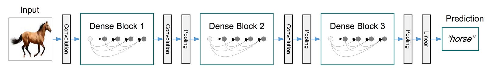
Each dense block contains the same number of composite layers. In the DenseNet all convolutions are performed with 3x3 kernels and "SAME" padding. Before the initial dense block a conventional layer with 16 output channels is performed. The sizes of the feature maps across the three dense blocks are 32x32, 16x16 and 8x8 respectively. The DenseNet configuration that I used is the (L=40 , K=12) or the 40 layer 12 growth factor version reported in the original paper. This configuration results in each dense block containing 12 composite layers
To reduce the generalisation gap and prevent over-fitting to training data regularisation strategies are typically used when training deep neural networks. After some experimentation with various regularisation techniques I found a set that were found to give good performance with both of the architectures considered
-
Dropout : Dropout provides an inexpensive approximation to training and evaluating a bagged ensemble of exponentially many neural networks. It does this by randomly setting some activations to zero in the layer it is applied to by a certain probably. The keep probabilities and locations of the dropout layers used for the two networks here are shown in the architecture descriptions above.
-
Batch Normalisation : Although batch normalisation was originally proposed as a strategy to reduce internal co-variate shift between the network layers to improve the speed and robustness of the training strategy, it has also been shown to give advantageous results for generalisation. This is thought to arise due to all training examples being seen in conjunction with other examples in the mini-batch, and the training network no longer producing deterministic values for a given training example.
-
Data Augmentation : Although not initially obvious, data augmentation is in itself a form of regularisation. From the notorious Deep Learning book by Goodfellow etal "Regularization is any modification we make to a learning algorithm that is intended to reduce its generalization error but not its training error". Augmenting the data is form of applying prior knowledge of the types of distortions it is likely to encounter and can thus be seen to reduce the model variance.
The two model architectures were trained on the augmented training data set and validated on the validation set during the training procedure to monitor how well the model is generalising to out of training set sample data. The training procedure for each network is described below. Both models were training using a Nvidia 1080 gt GPU
The Adam SGD based optimiser was chosen with a batch size of 128. The learning rate was initially chosen to be 1e-3. This was decreased after 40 epochs by a factor of 10, and repeated every 10 epochs after that. As this architecture is small the total computational time require was around 5 hours

As per the recommendations in the original DenseNet paper, the SGD optimiser with momentum set to 0.9 was chosen. As the dense architecture is very memory intensive the batch size was selected to be 64. The learning rate was set to 1e-3 for the first 30 epochs and the reduced by a factor of 10 for a further 10 epochs. The training time for the dense net architecture was substantially grater then the previously considered architecture and took around 22 hours in total. As the accuracy can be seen to slightly decrease towards the end of the DenseNet training, the final selected model was chosen to be at around 34 epochs, effectively using the early stopping strategy.

My final model results were:
- Training accuracy: 100 %
- Validation accuracy: 99.8%
- Test accuracy: 98.32 %
- Training accuracy: 100%
- Validation accuracy: 99.7%
- Test accuracy 99.02%
Now I have done the laborious task of building, training and testing two deep learning classification models on German traffic signs, it is time to test them in the wild to see how they perform. As I don't live in Germany, images of German traffic signs from the internet will have to do. I used google street view to walk the streets of Berlin and acquire 7 examples of traffic signs. These images were then resized to the appropriate sizes, prepossessed using the same methodology as before and then run through the two deep learning architectures to calculate the predicted class probabilities. These images and class probabilities are shown below


Both architectures considered correctly classified all 7 of the images giving them a both an effective accuracy of 100%. This agrees favourably with the accuracy found on the test set which was just below 100% accuracy with both models. Additionally all images tested with both models showed extremely high certainty of classification for the correct class (bar one example discussed below). It should be noted that all the images I found are quite easy to classify with clear visibility and small to no occlusion.
The only notable difference between the prediction accuracy of the two models was the 'keep right' example. This sign had some stickers on the face causing a small amount of occlusion. The AlexNet model still showed a near 100% probability of the correct sign, whilst the DenseNet was only 60% sure of this with a large amount of probability assigned to the second most likely class. This surprising result would suggest the AlexNet style architecture is more robust to the unwanted stickers compared with the higher test set scoring (and much more powerful) DenseNet model.
As further work I will look to analyse the classification performance of both these classification models in more detail using confusion matrices, precision, recall and f1 scores. I am unable to do this currently due to a busy work commitments.
Good accuracy results have been achieved using both considered architectures. I believe the DenseNet model could benefit from more data augmentation creating increasing the dataset size and also amount of distortion in each transform.